Machine learning algorithms have helped solve real-world problems as diverse as disease prediction and online shopping. However, many problems we would like to address with machine learning involve imbalanced datasets. In this chapter, we will discuss and define imbalanced datasets, explaining how they differ from other types of datasets. The ubiquity of imbalanced data will be demonstrated with examples of common problems and scenarios. We will also go through the basics of machine learning and cover the essentials, such as loss functions, regularization, and feature engineering. We will also learn about common evaluation metrics, particularly those that can be very helpful for imbalanced datasets. We will then introduce the imbalanced-learn library.

In particular, we will learn about the following topics:

• Introduction to imbalanced datasets
• Machine learning 101
• Types of datasets and splits
• Common evaluation metrics
• Challenges and considerations when dealing with imbalanced data
• When can we have an imbalance in datasets?
• Why can imbalanced data be a challenge?
• When to not worry about data imbalance
• Introduction to the imbalanced-learn library
• General rules to follow

In this chapter, we will utilize common libraries such as numpy and scikit-learn and introduce the imbalanced-learn library. The code and notebooks for this chapter are available on GitHub at https://github.com/PacktPublishing/Machine-Learning-for-Imbalanced-Data/tree/main/chapter01. You can fire up the GitHub notebook using Google Colab by clicking on the Open in Colab icon at the top of this chapter’s notebook or by launching it from https://colab.research.google.com using the GitHub URL of the notebook.

Machine learning algorithms learn from collections of examples that we call datasets. These datasets contain multiple data samples or points, which we may refer to as examples, samples, or instances interchangeably throughout this book.

A dataset can be said to have a balanced distribution when all the target classes have a similar number of examples, as shown in Figure 1.1:

Figure 1.1 – Balanced distribution with an almost equal number of examples for each class

Imbalanced datasets or skewed datasets are those that have some target classes (also called labels) that outnumber the rest of the classes (Figure 1.2). Though this generally applies to classification problems (for example, fraud detection) in machine learning, they inevitably occur in regression problems (for example, house price prediction) too:

Figure 1.2 – An imbalanced dataset with five classes and a varying number of samples

We label the class with more instances as the “majority” or “negative” class and the one with fewer instances as the “minority” or “positive” class. Most of the time, our main interest lies in the minority class, which is why we often refer to the minority class as the “positive” class and to the majority class as the “negative” class:

Figure 1.3 – A visual guide to common terminology used in imbalanced classification

This can be scaled to more than two classes, and such classification problems are called multi-class classification. In the first half of this book, we will focus our attention only on binary class classification to keep the material easier to grasp. It’s relatively easy to extend the concepts to multi-class classification.

Let’s look at a few examples of imbalanced datasets:

• Fraud detection is where fraudulent transactions need to be detected out of several transactions. This problem is often encountered and widely used in finance, healthcare, and e-commerce industries.
• Network intrusion detection using machine learning involves analyzing large volumes of network traffic data to detect and prevent instances of unauthorized access and misuse of computer systems.
• Cancer detection. Cancer is not rare, but we still may want to use machine learning to analyze medical data to identify potential cases of cancer earlier and improve treatment outcomes.

In this book, we would like to focus on the class imbalance problem in general and look at various solutions where we see that class imbalance is affecting the performance of our model. A typical problem is that models perform quite poorly on the minority classes for which the model has seen a very low number of examples during model training.

Let’s do a quick overview of machine learning and its related fields:

• Artificial intelligence is the superset of all intelligence-related problems. Classical machine learning encompasses problems that can be solved by training traditional classical models (such as decision trees or logistic regression) and predicting the target values. They typically work on tabular data, require extensive feature engineering (manual development of features), and are less effective on text and image data. Deep learning tends to do far better on image, text, speech, and video data, wherein, typically, no manual feature engineering is needed, and various layers in the neural network automatically do feature engineering for us.
• In supervised learning, we have both inputs and outputs (labels) in the dataset, and the model learns to predict the output during the training. Each input can be represented as a list of features. The output or labels can be a finite set of classes (classification), a real number (regression), or something more complex. A classic example of supervised learning in classification is the Iris flowers classification. In this case, the dataset includes features such as petal length, petal width, sepal length, and sepal width, and the labels are the species of the Iris flowers (setosa, versicolor, or virginica). A model can be trained on this dataset and then be used to classify new, unseen Iris flowers as one of these species.
• In unsupervised learning, models either don’t have access to the labels or don’t use the labels and then try to make some predictions – for example, clustering the examples in the dataset into different groups.
• In reinforcement learning, the model tries to learn by making mistakes and optimizing a goal or profit variable. An example would be training a model to play chess and adjusting its strategy based on feedback received through rewards and penalties.

In supervised learning (which is the focus of this book), there are two main types of problems: classification and regression. Classification problems involve categorizing data into predefined classes or labels, such as “fraud” or “non-fraud” and “spam” or “non-spam.” On the other hand, regression problems aim to predict a continuous variable, such as the price of a house.

While data imbalance can also affect regression problems, this book will concentrate solely on classification problems. This focus is due to several factors, such as the limited scope of this book and the well-established techniques available for classification. In some cases, you might even be able to reframe a regression problem as a classification problem, making the methods discussed in this book still relevant.

When it comes to various kinds of models that are popular for classification problems, we have quite a few categories of classical supervised machine learning models:

• Logistic regression: This is a supervised machine learning algorithm that’s used for binary classification problems. It predicts the probability of a binary target variable based on a set of predictor variables (features) by fitting a logistic function to the data, which outputs a value between 0 and 1.
• Support Vector Machines (SVMs): These are supervised machine learning algorithms that are mainly used for classification and can be extended to regression problems. SVMs classify data by finding the optimal hyperplane that maximally separates the different classes in the input data, thus making it a powerful tool for binary and multiclass classification tasks.
• K-Nearest Neighbors (KNN): This is a supervised machine learning algorithm that’s used for classification and regression analysis. It predicts the target variable based on the k-nearest neighbors in the training dataset. The value of k determines the number of neighbors to consider when making a prediction, and it can be tuned to optimize the model’s performance.
• Tree models: These are a type of supervised machine learning algorithm that’s used for classification and regression analysis. They recursively split the data into smaller subsets based on the most important features to create a decision tree that predicts the target variable based on the input features.
• Ensemble models: These combine multiple individual models to improve predictive accuracy and reduce overfitting (explained later in this chapter). Ensemble techniques include bagging (for example, random forest), boosting (for example, XGBoost), and stacking. They are commonly used for classification as well as regression analysis.
• Neural networks: These models are inspired by the human brain, consist of multiple layers with numerous neurons in each, and are capable of learning complex functions. We will discuss these in more detail in Chapter 6, Data Imbalance in Deep Learning.

Figure 1.4 displays the decision boundaries of various classifiers we have reviewed so far. It shows that logistic regression has a linear decision boundary, while tree-based models such as decision trees, random forests, and XGBoost work by dividing examples into axis-parallel rectangles to form their decision boundary. SVM, on the other hand, transforms the data to a different space so that it can plot its non-linear decision boundary. Neural networks have a non-linear decision boundary:

Figure 1.4 – The decision boundaries of popular machine learning algorithms on an imbalanced dataset

Next, we’ll delve into the principles underlying the process of model training.

What happens during model training?

In the training phase of a machine learning model, we provide a dataset consisting of examples, each with input features and a corresponding label, to the model. Let represent the list of features used for training, and be the list of labels in the training dataset. The goal of the model is to learn a function, , such that .

The model has adjustable parameters, denoted as θ, which are fine-tuned during the training process. The error function, commonly referred to as the loss function, is defined as . This error function needs to be minimized by a learning algorithm, which finds the optimal setting of these parameters, .

In classification problems, our typical loss functions are cross-entropy loss (also called the log loss):

Here, p is the predicted probability from the model when .

When the model’s prediction closely agrees with the target label, the loss function will approach zero. However, when the prediction deviates significantly from the target, the loss can become arbitrarily large, indicating a poor model fit.

As training progresses, the training loss keeps going down (Figure 1.5):

Figure 1.5 – Rate of change of the loss function as training progresses

This brings us to the concept of the fit of a model:

• A model is said to underfit if it is too simple and can’t capture the data’s complexity. It performs poorly on both training and new data.
• A model is of right fit if it accurately captures data patterns without learning noise. It performs well on both training and new data.
• An overfit model is too complex and learns noise along with data patterns. It performs well on training data but poorly on new data (Figure 1.6):

Figure 1.6 – Underfit, right fit, and overfit models for classification task

Next, let’s briefly try to learn about two important concepts in machine learning:

• Regularization is a set of techniques that are used to prevent the overfitting of a model to the training data. One type of regularization (namely L1 or L2) adds a penalty term to the loss function, which encourages the model to have smaller weights and reduces its complexity. This helps prevent the model from fitting too closely to the training data and generalizes better to unseen data.
• Feature engineering is the process of selecting and transforming the input features of a model to improve its performance. Feature engineering involves selecting the most relevant features for the problem, transforming them to make them more informative, and creating new features from the existing ones. Good feature engineering can make a huge difference in the performance of a model and can often be more important than the choice of algorithm or hyperparameters.

Typically, we train our model on the training set and test the model on an independent unseen dataset called the test set. We do this to do a fair evaluation of the model. If we don’t do this and train the model on the full dataset and evaluate the model on the same dataset, we don’t know how good the model would do on unseen data, plus the model will likely be overfitted.

We may encounter three kinds of datasets in machine learning:

• Training set: A dataset on which the model is trained.
• Validation set: A dataset used for tuning the hyperparameters of the model. A validation set is often referred to as a development set.
• Evaluation set or test set: A dataset used for evaluating the performance of the model.

When working with small example datasets, it’s common to allocate 80% of the data for the training set, 10% for the validation set, and 10% for the test set. However, the specific ratio between training and test sets is not as important as ensuring that the test set is large enough to provide statistically meaningful evaluation results. In the context of big data, a split of 98%, 1%, and 1% for training, validation, and test sets, respectively, could be appropriate.

Often, people don’t have a dedicated validation set for hyperparameter tuning and refer to the test set as an evaluation set. This can happen when the hyperparameter tuning is not performed as a part of the regular training cycle and is a one-off activity.

Cross-validation

Cross-validation can be a confusing term to guess its meaning. Breaking it down: cross + validation, so it’s some sort of validation on an extended (cross) something. Something here is the test set for us.

Let’s see what cross-validation is:

• Cross-validation is a technique that’s used to estimate how accurately a model will perform in practice
• It is typically used to detect overfitting – that is, failing to generalize patterns in data, particularly when the amount of data may be limited

Let’s look at the different types of cross-validation:

• Holdout: In the holdout method, we randomly assign data points to two sets, usually called the training set and the test set, respectively. We then train (build a model) on the training set and test (evaluate its performance) on the test set.
• k-fold: This works as follows:
  • We randomly shuffle the data.
  • We divide all the data into k parts, also known as folds. We train the model on k-1 folds and evaluate it on the remaining fold. We record the performance of this model using our chosen model evaluation metric, then discard this model.
  • We repeat this process k times, each time holding out a different subset for testing. We take an average of the evaluation metric values (for example, accuracy) from all the previous models. This average represents the overall performance measure of the model.

k-fold cross-validation is mainly used when you have limited data points, say 100 points. Using 5 or 10 folds is the most common when doing cross-validation.

Let’s look at the common evaluation metrics in machine learning, with a special focus on the ones relevant to problems with imbalanced data.

Several machine learning and deep learning metrics are used for evaluating the performance of classification models.

Let’s look at some of the helpful metrics that can help evaluate the performance of our model on the test set.

Confusion matrix

Given a model that tries to classify an example as belonging to the positive or negative class, there are four possibilities:

• True Positive (TP): This occurs when the model correctly predicts a sample as part of the positive class, which is its actual classification
• False Negative (FN): This happens when the model incorrectly classifies a sample from the positive class as belonging to the negative class
• True Negative (TN): This refers to instances where the model correctly identifies a sample as part of the negative class, which is its actual classification
• False Positive (FP): This occurs when the model incorrectly predicts a sample from the negative class as belonging to the positive class

Table 1.1 shows in what ways the model can get “confused” when making predictions, aptly called the confusion matrix. The confusion matrix forms the basis of many common metrics in machine learning:

Table 1.1 – Confusion matrix

Let’s look at some of the most common metrics in machine learning:

• True Positive Rate (TPR) measures the proportion of actual positive examples correctly classified by the model:

  

• False Positive Rate (FPR) measures the proportion of actual negative examples that are incorrectly identified as positives by the model:

  

• Accuracy: Accuracy is the fraction of correct predictions made out of all the predictions that the model makes. This is mathematically equal to . This functionality is available in the sklearn library as sklearn.metrics.accuracy_score.
• Precision: Precision, as an evaluation metric, measures the proportion of true positives over the number of items that the model predicts as belonging to the positive class, which is equal to the sum of the true positives and false positives. A high precision score indicates that the model has a low rate of false positives, meaning that when it predicts a positive result, it is usually correct. You can find this functionality in the sklearn library under the name sklearn.metrics.precision_score. .
• Recall (or sensitivity, or true positive rate): Recall measures the proportion of true positives over the number of items that belong to the positive class. The number of items that belong to the positive class is equal to the sum of true positives and false negatives. A high recall score indicates that the model has a low rate of false negatives, meaning that it correctly identifies most of the positive instances. It is especially important to measure recall when the cost of mislabeling a positive example as negative (false negatives) is high.

  Recall measures the model’s ability to correctly detect all the positive instances. Recall can be considered to be the accuracy of the positive class in binary classification. You can find this functionality in the sklearn library under the name sklearn.metrics.recall_score.

  Table 1.2 summarizes the differences between precision and recall:

Table 1.2 – Precision versus recall

Why can accuracy be a bad metric for imbalanced datasets?

Let’s assume we have an imbalanced dataset with 1,000 examples, with 100 labels belonging to class 1 (the minority class) and 900 belonging to class 0 (the majority class).

Let’s say we have a model that always predicts 0 for all examples. The model’s accuracy for the minority class is

Figure 1.7 – A comic showing accuracy may not always be the right metric

This brings us to the precision-recall trade-off in machine learning. Usually, precision and recall are inversely correlated – that is, when recall increases, precision most often decreases. Why? Note that recall and for recall to increase, FN should decrease. This means the model needs to classify more items as positive. However, if the model classifies more items as positive, some of these will likely be incorrect classifications, leading to an increase in the number of false positives (FPs). As the number of FPs increases, precision, defined as will decrease. With similar logic, you can argue that when recall decreases, precision often increases.

Next, let’s try to understand some of the precision and recall-based metrics that can help measure the performance of models trained on imbalanced data:

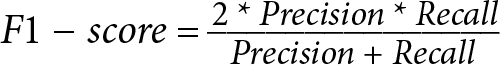
• F1 score: The F1 score (also called F-measure) is the harmonic mean of precision and recall. It combines precision and recall into a single metric. The F1 score varies between 0 and 1 and is most useful when we want to give equal priority to precision and recall (more on this later). This is available in the sklearn library as sklearn.metrics.f1_score.
• F-beta score or F-measure: The F-beta score is a generalization of the F1 score. It is a weighted harmonic mean of precision and recall, where the beta parameter controls the relative importance of precision and recall.

  The formula for the F-beta score is as follows:

  

  Here, beta is a positive parameter that determines the weight given to precision in the calculation of the score. When beta is set to 1, the F1 score is obtained, which is the harmonic mean of precision and recall. The F-beta score is a useful metric for imbalanced datasets, where one class may be more important than the other. By adjusting the beta parameter, we can control the relative importance of precision and recall for a particular class. For example, if we want to prioritize precision over recall for the minority class, we can set beta < 1. To see why that’s the case, set in the formula, which implies .

  Conversely, if we want to prioritize recall over precision for the minority class, we can set beta > 1 (we can set β = ∞ in the formula to see it reduce to recall).

  In practice, the choice of beta parameter depends on the specific problem and the desired trade-off between precision and recall. In general, higher values of beta result in more emphasis on recall, while lower values of beta result in more emphasis on precision. This is available in the sklearn library as sklearn.metrics.fbeta_score.

• Balanced accuracy score: The balanced accuracy score is defined as the average of the recall obtained in each class. This metric is commonly used in both binary and multiclass classification scenarios to address imbalanced datasets. This is available in the sklearn library as sklearn.metrics.balanced_accuracy_score.
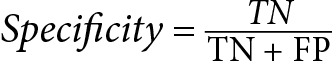
• Specificity (SPE): Specificity is a measure of the model’s ability to correctly identify the negative samples. In binary classification, it is calculated as the ratio of true negative predictions to the total number of negative samples. High specificity indicates that the model is good at identifying the negative class, while low specificity indicates that the model is biased toward the positive class.
• Support: Support refers to the number of samples in each class. Support is one of the values returned by the sklearn.metrics.precision_recall_fscore_support and imblearn.metrics.classification_report_imbalanced APIs.
• Geometric mean: The geometric mean is a measure of the overall performance of the model on imbalanced datasets. In imbalanced-learn, geometric_mean_score() is defined by the geometric mean of “accuracy on positive class examples” (recall or sensitivity or TPR) and “accuracy on negative class examples” (specificity or TNR). So, even if one class is heavily outnumbered by the other class, the metric will still be representative of the model’s overall performance.
• Index Balanced Accuracy (IBA): The IBA [1] is a measure of the overall accuracy of the model on imbalanced datasets. It takes into account both the sensitivity and specificity of the model and is calculated as the mean of the sensitivity and specificity, weighted by the imbalance ratio of each class. The IBA metric is useful for evaluating the overall performance of the model on imbalanced datasets and can be used to compare the performance of different models. IBA is one of the several values returned by imblearn.metrics.classification_report_imbalanced.

Table 1.3 shows the associated metrics and their formulas as an extension of the confusion matrix:

Table 1.3 – Confusion matrix with various metrics and their definitions

ROC

Receiver Operating Characteristics, commonly known as ROC curves, are plots that display the TPR on the y-axis against the FPR on the x-axis for various threshold values:

• The ROC curve essentially represents the proportion of correctly predicted positive instances on the y-axis, contrasted with the proportion of incorrectly predicted negative instances on the x-axis.
• In classification tasks, a threshold is a cut-off value that’s used to determine the class of an example. For instance, if a model classifies an example as “positive,” a threshold of 0.5 might be set to decide whether the instance should be labeled as belonging to the “positive” or “negative” class. The ROC curve can be used to identify the optimal threshold for a model. This topic will be discussed in detail in Chapter 5, Cost-Sensitive Learning.
• To create the ROC curve, we calculate the TPR and FPR for many various threshold values of the model’s predicted probabilities. For each threshold, the corresponding TPR value is plotted on the y-axis, and the FPR value is plotted on the x-axis, creating a single point. By connecting these points, we generate the ROC curve (Figure 1.8):

Figure 1.8 – The ROC curve as a plot of TPR versus FPR (the dotted line shows a model with no skill)

Some properties of the ROC curve are as follows:

• The Area Under Curve (AUC) of a ROC curve (also called AUC-ROC) serves a specific purpose: it provides a single numerical value that represents the model’s performance across all possible classification thresholds:
  • AUC-ROC represents the degree of separability of the classes. This means that the higher the AUC-ROC, the more the model can distinguish between the classes and predict a positive class example as positive and a negative class example as negative. A poor model with an AUC near 0 essentially predicts a positive class as a negative class and vice versa.
  • The AUC-ROC of a random classifier is 0.5 and is the diagonal joining the points (0,0) and (1,0) on the ROC curve.
  • The AUC-ROC has a probabilistic interpretation: an AUC of 0.9 indicates a 90% likelihood that the model will assign a higher score to a randomly chosen positive class example than to a negative class example. That is, AUC-ROC can be depicted as follows:

P(score(x+ ) > score(x− ))

Here, 𝑥+ denotes the positive (minority) class, and 𝑥− denotes the negative (majority) class.

• In the context of evaluating model performance, it’s crucial to use a test set that reflects the distribution of the data the model will encounter in real-world scenarios. This is particularly relevant when considering metrics such as the ROC curve, which remains consistent regardless of changes in class imbalance within the test data. Whether we have 1:1, 1:10, or 1:100 as the minority_class: majority_class distribution in the test set, the ROC curve remains the same [2]. The reason for this is that both of these rates are independent of the class distribution in the test data because they are calculated only based on the correctly and incorrectly classified instances of each class, not the total number of instances of each class. This is not to be confused with the change in imbalance in the training data, which can adversely impact the model’s performance and would be reflected in the ROC curve.

Now, let’s look at some of the problems in using ROC for imbalanced datasets:

• ROC does not distinguish between the various classes – that is, it does not emphasize one class more over the other. This can be a problem for imbalanced datasets where, often, the minority class is more important to detect than the majority class. Because of this, it may not reflect the minority class well. For example, we may want better recall over precision.
• While ROC curves can be useful for comparing the performance of models across a full range of FPRs, they may not be as relevant for specific applications that require a very low FPR, such as fraud detection in financial transactions or banking applications. The reason the FPR needs to be very low is that such applications usually require limited manual intervention. The number of transactions that can be manually checked may be as low as 1% or even 0.1% of all the data, which means the FPR can’t be higher than 0.001. In these cases, anything to the right of an FPR equal to 0.001 on the ROC curve becomes irrelevant [3]. To further understand this point, let’s consider an example:
  • Let’s say that for a test set, we have a total of 10,000 examples and only 100 examples of the positive class, making up 1% of the examples. So, any FPR higher than 1% - that is, 0.01 – is going to raise too many alerts to be handled manually by investigators.
  • The performance on the far left-hand side of the ROC curve becomes crucial in most real-world problems, which are often dominated by a large number of negative instances. As a result, most of the ROC curve becomes irrelevant for applications that need to maintain a very low FPR.

Precision-Recall curve

Similar to ROC curves, Precision-Recall (PR) curves plot a pair of metrics for different threshold values. But unlike ROC curves, which plot TPR and FPR, PR curves plot precision and recall. To demonstrate the difference between the two curves, let’s say we compare the performance of two models – Model 1 and Model 2 – on a particular handcrafted imbalanced dataset:

• In Figure 1.9 (a), the ROC curves for both models appear to be close to the top-left corner (point (0, 1)), which might lead you to conclude that both models are performing well. However, this can be misleading, especially in the context of imbalanced datasets.
• When we turn our attention to the PR curves in Figure 1.9 (b), a different story unfolds. Model 2 comes closer to the ideal top-right corner (point (1, 1)) of the plot, indicating that its performance is much better than Model 1 when precision and recall are considered.
• The PR curve reveals that Model 2 has an advantage over Model 1.

This discrepancy between the ROC and PR curves also underscores the importance of using multiple metrics for model evaluation, particularly when dealing with imbalanced data:

Figure 1.9 – The PR curve can show obvious differences between models compared to the ROC curve

Let’s try to understand these observations in detail. While the ROC curve shows very little difference between the performance of the two models, the PR curve shows a much bigger gap. The reason for this is that the ROC curve uses FPR, which is FP/(FP+TN). Usually, TN is really high for an imbalanced dataset, and hence even if FP changes by a decent amount, FPR’s overall value is overshadowed by TN. Hence, ROC doesn’t change by a whole lot.

The conclusion of which classifier is superior can change with the distribution of classes in the test set. In the case of skewed datasets, the PR curve can more clearly show that the model did not work well compared to the ROC curve, as shown in the preceding figure.

The average precision is a single number that’s used to summarize a PR curve, and the corresponding API in sklearn is sklearn.metrics.average_precision_score.

Relation between the ROC curve and PR curve

The primary distinction between the ROC curve and the PR curve lies in the fact that while ROC assesses how well the model can “calculate” both positive and negative classes, PR solely focuses on the positive class. Therefore, when dealing with a balanced dataset scenario and you are concerned with both the positive and negative classes, ROC AUC works exceptionally well. In contrast, when dealing with an imbalanced situation, PR AUC is more suitable. However, it’s important to keep in mind that PR AUC only evaluates the model’s ability to “calculate” the positive class. Because PR curves are more sensitive to the positive (minority) class, we will be using PR curves throughout the first half of this book.

We can reimagine the PR curve with precision on the x-axis and TPR, also known as recall, on the y-axis. The key difference between the two curves is that while the ROC curve uses FPR, the PR curve uses precision.

As discussed earlier, FPR tends to be very low when dealing with imbalanced datasets. This aspect of having low FPR values is crucial in certain applications such as fraud detection, where the capacity for manual investigations is inherently limited. Consequently, this perspective can alter the perceived performance of classifiers. As shown in Figure 1.9, it’s also possible that the performances of the two models seem reversed when compared using average precision (0.69 versus 0.90) instead of AUC-ROC (0.97 and 0.95).

Let’s summarize this:

• The AUC-ROC is the area under the curve plotted with TPR on the y-axis and FPR on the x-axis.
• The AUC-PR is the area under the curve plotted with precision on the y-axis and recall on the x-axis.

As TPR equals recall, the two plots only differ in what recall is compared to – either precision or FPR. Additionally, the plots are rotated by 90 degrees relative to each other:

Table 1.4 – Comparing the ROC and PR curves

In the next few sections, we’ll explore the circumstances that lead to imbalances in datasets, the challenges these imbalances can pose, and the situations where data imbalance might not be a concern.

In certain instances, directly using data for machine learning without worrying about data imbalance can yield usable results suitable for a given business scenario. Yet, there are situations where a more dedicated effort is needed to manage the effects of imbalanced data.

Broad statements claiming that you must always or never adjust for imbalanced classes tend to be misleading. The truth is that the need to address class imbalance is contingent on the specific characteristics of the data, the problem at hand, and the definition of an acceptable solution. Therefore, the approach to dealing with class imbalance should be tailored according to these factors.

In this section, we’ll explore various situations and causes leading to an imbalance in datasets, such as rare event occurrences or skewed data collection processes:

• Inherent in the problem: Sometimes, the task we need to solve involves detecting outliers in datasets – for example, patients with a certain disease or fraud cases in a set of transactions. In such cases, the dataset is inherently imbalanced because the target events are rare to begin with.
• High cost of data collection while bootstrapping a machine learning solution: The cost of collecting data might be too high for certain classes. For example, collecting data on COVID-19 patients incurs high costs due to the need for specialized medical tests, protective equipment, and the ethical and logistical challenges of obtaining informed consent in a high-stress healthcare environment.
• Noisy labels for certain classes: This may happen when a lot of noise is introduced into the labels of the dataset for certain classes during data collection.
• Labeling errors: Errors in labeling can also contribute to data imbalance. For example, if some samples are mistakenly labeled as negative when they are positive, this can result in an imbalance in the dataset. Additionally, if a class is already inherently rare, human annotators might be biased and overlook the few examples of that rare class that do exist.
• Sampling bias: Data collection methods can sometimes introduce bias in the dataset. For example, if a survey is conducted in a specific geographical area or among a specific group of people, the resulting dataset may not be representative of the entire population.
• Data cleaning: During the data cleaning or filtering process, some classes or samples may be removed due to incomplete or missing data. This can result in an imbalance in the remaining dataset.

Let’s delve into the difficulties posed by imbalanced data on model predictions and their impact on model performance:

• Failure of metrics such as accuracy: As we discussed previously, conventional metrics such as accuracy can be misleading in the context of imbalanced data (a 99% imbalanced dataset would still achieve 99% accuracy). Threshold-invariant metrics such as the PR curve or ROC curve attempt to expose the performance of the model over a wide range of thresholds. The real challenge lies in the disproportionate influence of the “true negative” cell in the confusion matrix. Metrics that focus less on “true negatives,” such as precision, recall, or F1 score, are more appropriate for evaluating model performance. It’s important to note that these metrics have a hidden hyperparameter – the classification threshold – that should not be ignored but optimized for real-world applications (refer to Chapter 5, Cost-Sensitive Learning, to learn more about threshold tuning).
• Imbalanced data can be a challenge for a model’s loss function: This may happen because the loss function is typically designed to minimize the errors between the predicted outputs and the true labels of the training data. When the data is imbalanced, there are more instances of one class than another, and the model may become biased toward the majority class. We will discuss solutions to this issue in more detail in Chapter 5, Cost-Sensitive Learning, and Chapter 8, Algorithm-Level Deep Learning Techniques.
• Different misclassification costs for different classes: Often, it may be more expensive to misclassify positive examples than to misclassify negative examples. We may have false positives that are more expensive than false negatives. For example, usually, the cost of misclassifying a patient with cancer as healthy (false negative) will be much higher than misclassifying a healthy patient as having cancer (false positive). Why? Because it’s much cheaper to go through some extra tests to revalidate the test results in the second case instead of detecting it much later in the first case. This is called the cost of misclassification, which could be different for the majority and minority classes, making things complicated for imbalanced datasets. We will discuss more about this in Chapter 5, Cost-Sensitive Learning.
• Constraints on computational resources: In sectors such as finance, healthcare, and retail, handling big data is a common challenge. Training on these large datasets is not only time-consuming but also costly due to the computational power needed. In such scenarios, downsampling or undersampling the majority class becomes essential, as will be discussed in Chapter 3, Undersampling Methods. Additionally, acquiring more samples for the minority class can further increase dataset size and computational costs. Memory limitations may also restrict the amount of data that can be processed.
• Not enough variation in the minority class examples to sufficiently represent its distribution: Often, an absolute number of samples of the minority class is not as big of a problem as the variation in the samples of the minority class. The dataset might look large, but there might not be many variations or varieties in the samples that adequately represent the distribution of minority classes. This can lead to the model not being able to learn the classification boundary properly, which would lead to poor performance of the model (Figure 1.10). This can often happen in computer vision problems, such as object detection, where we may have very few samples of certain classes. In such cases, data augmentation techniques (discussed in Chapter 7, Data-Level Deep Learning Methods) can help significantly:

Figure 1.10 – Change in decision boundary with a different distribution of minority class examples – the crosses denote the majority class, and the circles denote the minority class

• Poor performance of uncalibrated models: Imbalanced data can be a challenge for uncalibrated models. Uncalibrated models are models that do not output well-calibrated probabilities, which means that the predicted probabilities may not reflect the true likelihood of the predicted classes:
  • When dealing with imbalanced data, uncalibrated models can be particularly susceptible to producing biased predictions toward the majority class as they may not be able to effectively differentiate between the minority and majority classes. This can lead to poor performance in the minority class, where the model may produce overly confident predictions or predictions that are too conservative.
  • For example, an uncalibrated model that is trained on imbalanced data may incorrectly classify instances that belong to the minority class as majority class examples, often with high confidence. This is because the model may not have learned to adjust its predictions based on the imbalance in the data and may not have a good understanding of the minority class examples.
  • To address this challenge, it is important to use well-calibrated models [4] that can output probabilities that reflect the true likelihood of the predicted classes. This can be achieved through techniques such as Platt scaling or isotonic regression, which can calibrate the predicted probabilities of an uncalibrated model to produce more accurate and reliable probabilities. Model calibration will be discussed in detail in Chapter 10, Model Calibration.
• Poor performance of models because of non-adjusted thresholds: It’s important to use intelligent thresholding when making predictions using models trained on imbalanced datasets. Simply predicting 1 when the model probability is over 0.5 may not always be the best approach. Instead, we should consider other thresholds that may be more effective. This can be achieved by examining the PR curve of the model rather than relying solely on its success rate with a default probability threshold of 0.5. Threshold adjustment can be quite important, even for models trained on naturally or artificially balanced datasets. We will discuss threshold adjustment in detail in Chapter 5, Cost-Sensitive Learning.

Next, let’s try to see when we shouldn’t do anything about data imbalance.

Class imbalance may not always negatively impact performance, and using imbalance-specific methods can sometimes worsen results [5]. Therefore, it’s crucial to accurately assess whether a task is genuinely affected by class imbalance before applying any specialized techniques. One such strategy can be as simple as setting up a baseline model without worrying about class imbalance and observing the model’s performance on various classes using various performance metrics.

Let’s explore scenarios where data imbalance may not be a concern and no corrective measures may be needed:

• When the imbalance is small: If the imbalance in the dataset is relatively small, with the ratio of the minority class to the majority class being only slightly skewed (say 4:5 or 2:3), the impact on the model’s performance may be minimal. In such cases, the model may still perform reasonably well without requiring any special techniques to handle the imbalance.
• When the goal is to predict the majority class: In some cases, the focus may be on predicting the majority class accurately, and the minority class may not be of particular interest. For example, in online ad placement, the focus can be on targeting users (majority class) likely to click on ads to maximize click-through rates and immediate revenue, while less attention is given to users (minority class) who may find ads annoying.
• When the cost of misclassification is nearly equal for both classes: In some applications, the cost of misclassifying a positive class example is not high (that is, false negative). An example is classifying emails as spam or non-spam. It’s totally fine to miss a spam email once in a while and misclassify it as non-spam. In such cases, the impact of misclassification on the performance metrics may be negligible, and the imbalance may not be a concern.
• When the dataset is sufficiently large: Even if the ratio of minority to majority class samples is very low, such as 1:100, and if the dataset is sufficiently large, with a large number of samples in both the minority and majority classes, the impact of data imbalance on the model’s performance may be reduced. With a larger dataset, the model may be able to learn the patterns in the minority class more effectively. However, it would still be advisable to compare the baseline model’s performance with the performance of models that take the data imbalance into account. For example, compare a baseline model to models with threshold adjustment, oversampling, and undersampling (Chapter 2, Oversampling Methods, and Chapter 3, Undersampling Methods), and algorithm-based techniques such as cost-sensitive learning (Chapter 5, Cost-Sensitive Learning).

In the next section, we will become familiar with a library that can be very useful when dealing with imbalanced data. We will train a model on an imbalanced toy dataset and look at some metrics to evaluate the performance of the trained model.

imbalanced-learn (imported as imblearn) is a Python package that offers several techniques to deal with data imbalance. In the first half of this book, we will rely heavily on this library. Let’s install the imbalanced-learn library:

pip3 install imbalanced-learn==0.11.0

We can use imbalanced-learn to create a synthetic dataset for our analysis:

from sklearn.datasets import make_classification
import pandas as pd
import matplotlib.pyplot as plt
import seaborn as sns
def make_data(sep):
    X, y = make_classification(n_samples=50000,
        n_features=2, n_redundant=0,
        n_clusters_per_class=1, weights=[0.995],
        class_sep=sep, random_state=1)
    X = pd.DataFrame(X, columns=['feature_1', 'feature_2'])
    y = pd.Series(y)
    return X, y

Let’s analyze the generated dataset:

from collections import Counter
X, y = make_data(sep=2)
print(y.value_counts())
sns.scatterplot(data=X, x="feature_1", y="feature_2", hue=y)
plt.title('Separation: {}'.format(separation))
plt.show()

Here’s the output:

0     49498
1       502

Figure 1.11 – 2 class dataset with two features

Let’s split this dataset into training and test sets:

From sklearn.model_selection import train_test_split
X_train, X_test, y_train, y_test = train_test_split(X, y, stratify = \
    y, test_size=0.2, random_state=42)
print('train data: ', Counter(y_train))
print('test data: ', Counter(y_test))

Here’s the output:

train data:  Counter({0: 39598, 1: 402})
test data:  Counter({0: 9900, 1: 100})

Note the usage of stratify in the train_test_split API of sklearn. Specifying stratify=y ensures we maintain the same ratio of majority and minority classes in both the training set and the test set. Let’s understand stratification in more detail.

Stratified sampling is a way to split the dataset into various subgroups (called “strata”) based on certain characteristics they share. It can be highly valuable when dealing with imbalanced datasets because it ensures that the train and test datasets have the same proportions of class labels as the original dataset.

In an imbalanced dataset, the minority class constitutes a small fraction of the total data. If we perform a simple random split without any stratification, there’s a risk that the minority class may not be adequately represented in the training set or could be entirely left out from the test set, which may lead to poor performance and unreliable evaluation metrics.

With stratified sampling, the proportion of each class in the overall dataset is preserved in both training and test sets, ensuring representative sampling and a better chance for the model to learn from the minority class. This leads to a more robust model and a more reliable evaluation of the model’s performance.

The scikit-learn APIs for stratification

The scikit-learn APIs, such as RepeatedStratifiedKFold and StratifiedKFold, employ the concept of stratification to evaluate model performance through cross-validation, especially when working with imbalanced datasets.

Now, let’s train a logistic regression model on training data:

from sklearn.linear_model import LogisticRegression
lr = LogisticRegression(random_state=0, max_iter=2000)
lr.fit(X_train, y_train)
y_pred = lr.predict(X_test)

Let’s get the report metrics from the sklearn library:

from sklearn.metrics import classification_report
print(classification_report(y_test, y_pred))

This outputs the following:

          precision     recall      f1-score    support
0         0.99          1.00        1.00        9900
1         0.94          0.17        0.29        100
accuracy                                0.99      10000
macro avg       0.97        0.58        0.64      10000
weighted avg    0.99        0.99        0.99      10000

Let’s get the report metrics from imblearn:

from imblearn.metrics import classification_report_imbalanced
print(classification_report_imbalanced(y_test, y_pred))

This outputs a lot more columns:

Figure 1.12 – Output of the classification report from imbalanced-learn

Do you notice the extra metrics here compared to the API of sklearn? We got three additional metrics: spe for specificity, geo for geometric mean, and iba for index balanced accuracy.

The imblearn.metrics module has several such functions that can be helpful for imbalanced datasets. Apart from classification_report_imbalanced(), it offers APIs such as sensitivity_specificity_support(), geometric_mean_score(), sensitivity_score(), and specificity_score().

Usually, the first step in any machine learning pipeline should be to split the data into train/test/validation sets. We should avoid applying any techniques to handle the imbalance until after the data has been split. We should begin by splitting the data into training, testing, and validation sets and then proceed with any necessary adjustments to the training data. Applying techniques such as oversampling (see Chapter 2, Oversampling Methods) before splitting the data can result in data leakage, overfitting, and over-optimism [6].

We should ensure that the validation data closely resembles the test data. Both validation data and test data should represent real-world scenarios on which the model will be used for prediction. Avoid applying any sampling techniques or modifications to the validation set. The only requirement is to include a sufficient number of samples from all classes.

Let’s switch to discussing a bit about using unsupervised learning algorithms. Anomaly detection or outlier detection is a class of problems that can be used for dealing with imbalanced data problems. Anomalies or outliers are data points that deviate significantly from the rest of the data. These anomalies often correspond to the minority class in an imbalanced dataset, making unsupervised methods potentially useful.

The term that’s often used for these kinds of problems is one-class classification. This technique is particularly beneficial when the positive (minority) cases are sparse or when gathering them before the training is not feasible. The model is trained exclusively on what is considered the “normal” or majority class. It then classifies new instances as “normal” or “anomalous,” effectively identifying what could be the minority class. This can be especially useful for binary imbalanced classification problems, where the majority class is deemed “normal,” and the minority class is considered an anomaly.

However, it does have a drawback: outliers or positive cases during training are discarded [7], which could lead to the potential loss of valuable information.

In summary, while unsupervised methods such as one-class classification offer an alternative for managing class imbalance, our discussion in this book will remain centered on supervised learning algorithms. Nevertheless, we recommend that you explore and experiment with such solutions when you find them appropriate.

Let’s summarize what we’ve learned so far. Imbalanced data is a common problem in machine learning, where there are significantly more instances of one class than another. Imbalanced datasets can arise from various situations, including rare event occurrences, high data collection costs, noisy labels, labeling errors, sampling bias, and data cleaning. This can be a challenge for machine learning models as they may be biased toward the majority class.

Several techniques can be used to deal with imbalanced data, such as oversampling, undersampling, and cost-sensitive learning. The best technique to use depends on the specific problem and the data.

In some cases, data imbalance may not be a concern. When the dataset is sufficiently large, the impact of data imbalance on the model’s performance may be reduced. However, it is still advisable to compare the baseline model’s performance with the performance of models that have been built using techniques that address data imbalance, such as threshold adjustment, data-based techniques (oversampling and undersampling), and algorithm-based techniques.

Traditional performance metrics such as accuracy can fail in imbalanced datasets. Some more useful metrics for imbalanced datasets are the ROC curve, the PR curve, precision, recall, and F1 score. While ROC curves are suitable for balanced datasets, PR curves are more suitable for imbalanced datasets when one class is more important than the other.

The imbalanced-learn library is a Python package that offers several techniques to deal with data imbalance.

There are some general rules to follow, such as splitting the data into train/test/validation sets before applying any techniques to handle the imbalance in the data, ensuring that the validation data closely resembles the test data and that test data represents the data on which the model will make final predictions, and avoiding applying any sampling techniques or modifications to the validation set and test set.

One-class classification or anomaly detection is another technique that can be used for dealing with unsupervised imbalanced data problems. In this book, we will focus our discussion on supervised learning algorithms only.

In the next chapter, we will look at one of the common ways to handle the data imbalance problem in datasets by applying oversampling techniques.

1. How does the choice of loss function when training a model affect the performance of the model on imbalanced datasets?
2. Can you explain why the PR curve is more informative than the ROC curve when dealing with highly skewed datasets?
3. What are some of the potential issues with using accuracy as a metric for model performance on imbalanced datasets?
4. How does the concept of “class imbalance” affect the process of feature engineering in machine learning?
5. In the context of imbalanced datasets, how does the choice of “k” in k-fold cross-validation affect the performance of the model? How would you fix the issue?
6. How does the distribution of classes in the test data affect the PR curve, and why? What about the ROC curve?
7. What are the implications of having a high AUC-ROC but a low AUC-PR in the context of an imbalanced dataset?
8. How does the concept of “sampling bias” contribute to the challenge of imbalanced datasets in machine learning?
9. How does the concept of “labeling errors” contribute to the challenge of imbalanced datasets in machine learning?
10. What are some of the real-world scenarios where dealing with imbalanced datasets is inherently part of the problem?
11. Matthews Correlation Coefficient (MCC) is a metric that takes all the cells of the confusion matrix into account and is given by the following formula:

    

    1. What can be the minimum and maximum values of the metric?
    2. Because it takes TN into account, its value may not change much when we are comparing different models, but it can tell us if the predictions for various classes are going well. Let’s illustrate this through an artificial example where we take a dummy model that always predicts 1 for an imbalanced test set made of 100 examples, with 90 of class 1 and 10 of class 0. Compute the various terms in the MCC formula and the value of MCC. Also, compute the values of accuracy, precision, recall, and F1 score.
    3. What can you conclude about the model from the MCC value that you just computed in the previous question?
    4. Create an imbalanced dataset using imblearn’s fetch_dataset API and then compute the values of MCC, accuracy, precision, recall, and F1 score. See if the MCC value can be a useful metric for this dataset.

1. V. García, R. A. Mollineda, and J. S. Sánchez, Index of Balanced Accuracy: A Performance Measure for Skewed Class Distributions, in Pattern Recognition and Image Analysis, vol. 5524, H. Araujo, A. M. Mendonça, A. J. Pinho, and M. I. Torres, Eds. Berlin, Heidelberg: Springer Berlin Heidelberg, 2009, pp. 441–448. Accessed: Mar. 18, 2023. [Online]. Available at http://link.springer.com/10.1007/978-3-642-02172-5_57.
2. T. Fawcett, An introduction to ROC analysis, Pattern Recognition Letters, vol. 27, no. 8, pp. 861–874, Jun. 2006, doi: 10.1016/j.patrec.2005.10.010.
3. Y.-A. Le Borgne, W. Siblini, B. Lebichot, and G. Bontempi, Reproducible Machine Learning for Credit Card Fraud Detection - Practical Handbook. Université Libre de Bruxelles, 2022. [Online]. Available at https://github.com/Fraud-Detection-Handbook/fraud-detection-handbook.
4. W. Siblini, J. Fréry, L. He-Guelton, F. Oblé, and Y.-Q. Wang, Master your Metrics with Calibration, vol. 12080, 2020, pp. 457–469. doi: 10.1007/978-3-030-44584-3_36.
5. Xu-Ying Liu, Jianxin Wu, and Zhi-Hua Zhou, Exploratory Undersampling for Class-Imbalance Learning, IEEE Trans. Syst., Man, Cybern. B, vol. 39, no. 2, pp. 539–550, Apr. 2009, doi: 10.1109/TSMCB.2008.2007853.
6. M. S. Santos, J. P. Soares, P. H. Abreu, H. Araujo, and J. Santos, Cross-Validation for Imbalanced Datasets: Avoiding Overoptimistic and Overfitting Approaches [Research Frontier], IEEE Comput. Intell. Mag., vol. 13, no. 4, pp. 59–76, Nov. 2018, doi: 10.1109/MCI.2018.2866730.
7. A. Fernández, S. García, M. Galar, R. Prati, B. Krawczyk, and F. Herrera, Learning from Imbalanced Data Sets. Springer International Publishing, 2018