Most of us started our machine learning (ML) journey by training our first ML model using a sample dataset on our laptops or home computers. Things are somewhat straightforward until we need to work with much larger datasets and run our ML experiments in the cloud. It also becomes more challenging once we need to deploy our trained models to production-level inference endpoints or web servers. There are a lot of things to consider when designing and building ML systems and these are just some of the challenges data scientists and ML engineers face when working on real-life requirements. That said, we must use the right platform, along with the right set of tools, when performing ML experiments and deployments in the cloud.

At this point, you might be wondering why we should even use a cloud platform when running our workloads. Can’t we build this platform ourselves? Perhaps you might be thinking that building and operating your own data center is a relatively easy task. In the past, different teams and companies have tried setting up infrastructure within their data centers and on-premise hardware. Over time, these companies started migrating their workloads to the cloud as they realized how hard and expensive it was to manage and operate data centers. A good example of this would be the Netflix team, which migrated their resources to the AWS cloud. Migrating to the cloud allowed them to scale better and allowed them to have a significant increase in service availability.

The Amazon Web Services (AWS) platform provides a lot of services and capabilities that can be used by professionals and companies around the world to manage different types of workloads in the cloud. These past couple of years, AWS has announced and released a significant number of services, capabilities, and features that can be used for production-level ML experiments and deployments as well. This is due to the increase in ML workloads being migrated to the cloud globally. As we go through each of the chapters in this book, we will have a better understanding of how different services are used to solve the challenges when productionizing ML models.

The following diagram shows the hands-on journey for this chapter:

Figure 1.1 – Hands-on journey for this chapter

In this introductory chapter, we will focus on getting our feet wet by trying out different options when building an ML model on AWS. As shown in the preceding diagram, we will use a variety of AutoML services and solutions to build ML models that can help us predict if a hotel booking will be cancelled or not based on the information available. We will start by setting up a Cloud9 environment, which will help us run our code through an integrated development environment (IDE) in our browser. In this environment, we will generate a realistic synthetic dataset using a deep learning model called the Conditional Generative Adversarial Network. We will upload this dataset to Amazon S3 using the AWS CLI. Inside the Cloud9 environment, we will also install AutoGluon and run an AutoML experiment to train and generate multiple models using the synthetic dataset. Finally, we will use SageMaker Canvas and SageMaker Autopilot to run AutoML experiments using the uploaded dataset in S3. If you are wondering what these fancy terms are, keep reading as we demystify each of these in this chapter.

In this chapter, we will cover the following topics:

• What is expected from ML engineers?
• How ML engineers can get the most out of AWS
• Essential prerequisites
• Preparing the dataset
• AutoML with AutoGluon
• Getting started with SageMaker and SageMaker Canvas
• No-code machine learning with SageMaker Canvas
• AutoML with SageMaker Autopilot

In addition to getting our feet wet using key ML services, libraries, and tools to perform AutoML experiments, this introductory chapter will help us gain a better understanding of several ML and ML engineering concepts that will be relevant to the succeeding chapters of this book. With this in mind, let’s get started!

Before we start, we must have an AWS account. If you do not have an AWS account yet, simply create an account here: https://aws.amazon.com/free/. You may proceed with the next steps once the account is ready.

The Jupyter notebooks, source code, and other files for each chapter are available in this book’s GitHub repository: https://github.com/PacktPublishing/Machine-Learning-Engineering-on-AWS.

ML engineering involves using ML and software engineering concepts and techniques to design, build, and manage production-level ML systems, along with pipelines. In a team working to build ML-powered applications, ML engineers are generally expected to build and operate the ML infrastructure that’s used to train and deploy models. In some cases, data scientists may also need to work on infrastructure-related requirements, especially if there is no clear delineation between the roles and responsibilities of ML engineers and data scientists in an organization.

There are several things an ML engineer should consider when designing and building ML systems and platforms. These would include the quality of the deployed ML model, along with the security, scalability, evolvability, stability, and overall cost of the ML infrastructure used. In this book, we will discuss the different strategies and best practices to achieve the different objectives of an ML engineer.

ML engineers should also be capable of designing and building automated ML workflows using a variety of solutions. Deployed models degrade over time and model retraining becomes essential in ensuring the quality of deployed ML models. Having automated ML pipelines in place helps enable automated model retraining and deployment.

Important note

If you are excited to learn more about how to build custom ML pipelines on AWS, then you should check out the last section of this book: Designing and building end-to-end MLOps pipelines. You should find several chapters dedicated to deploying complex ML pipelines on AWS!

There are many services and capabilities in the AWS platform that an ML engineer can choose from. Professionals who are already familiar with using virtual machines can easily spin up EC2 instances and run ML experiments using deep learning frameworks inside these virtual private servers. Services such as AWS Glue, Amazon EMR, and AWS Athena can be utilized by ML engineers and data engineers for different data management and processing needs. Once the ML models need to be deployed into dedicated inference endpoints, a variety of options become available:

Figure 1.2 – AWS machine learning stack

As shown in the preceding diagram, data scientists, developers, and ML engineers can make use of multiple services and capabilities from the AWS machine learning stack. The services grouped under AI services can easily be used by developers with minimal ML experience. To use the services listed here, all we need would be some experience working with data, along with the software development skills required to use SDKs and APIs. If we want to quickly build ML-powered applications with features such as language translation, text-to-speech, and product recommendation, then we can easily do that using the services under the AI Services bucket. In the middle, we have ML services and their capabilities, which help solve the more custom ML requirements of data scientists and ML engineers. To use the services and capabilities listed here, a solid understanding of the ML process is needed. The last layer, ML frameworks and infrastructure, offers the highest level of flexibility and customizability as this includes the ML infrastructure and framework support needed by more advanced use cases.

So, how can ML engineers make the most out of the AWS machine learning stack? The ability of ML engineers to design, build, and manage ML systems improves as they become more familiar with the services, capabilities, and tools available in the AWS platform. They may start with AI services to quickly build AI-powered applications on AWS. Over time, these ML engineers will make use of the different services, capabilities, and infrastructure from the lower two layers as they become more comfortable dealing with intermediate ML engineering requirements.

In this section, we will prepare the following:

• The Cloud9 environment
• The S3 bucket
• The synthetic dataset, which will be generated using a deep learning model

Let’s get started.

Creating the Cloud9 environment

One of the more convenient options when performing ML experiments inside a virtual private server is to use the AWS Cloud9 service. AWS Cloud9 allows developers, data scientists, and ML engineers to manage and run code within a development environment using a browser. The code is stored and executed inside an EC2 instance, which provides an environment similar to what most developers have.

Important note

It is recommended to use an Identity and Access Management (IAM) user with limited permissions instead of the root account when running the examples in this book. We will discuss this along with other security best practices in detail in Chapter 9, Security, Governance, and Compliance Strategies. If you are just starting to use AWS, you may proceed with using the root account in the meantime.

Follow these steps to create a Cloud9 environment where we will generate the synthetic dataset and run the AutoGluon AutoML experiment:

1. Type cloud9 in the search bar. Select Cloud9 from the list of results:

Figure 1.3 – Navigating to the Cloud9 console

Here, we can see that the region is currently set to Oregon (us-west-2). Make sure that you change this to where you want the resources to be created.

2. Next, click Create environment.
3. Under the Name environment field, specify a name for the Cloud9 environment (for example, mle-on-aws) and click Next step.
4. Under Environment type, choose Create a new EC2 instance for environment (direct access). Select m5.large for Instance type and then Ubuntu Server (18.04 LTS) for Platform:

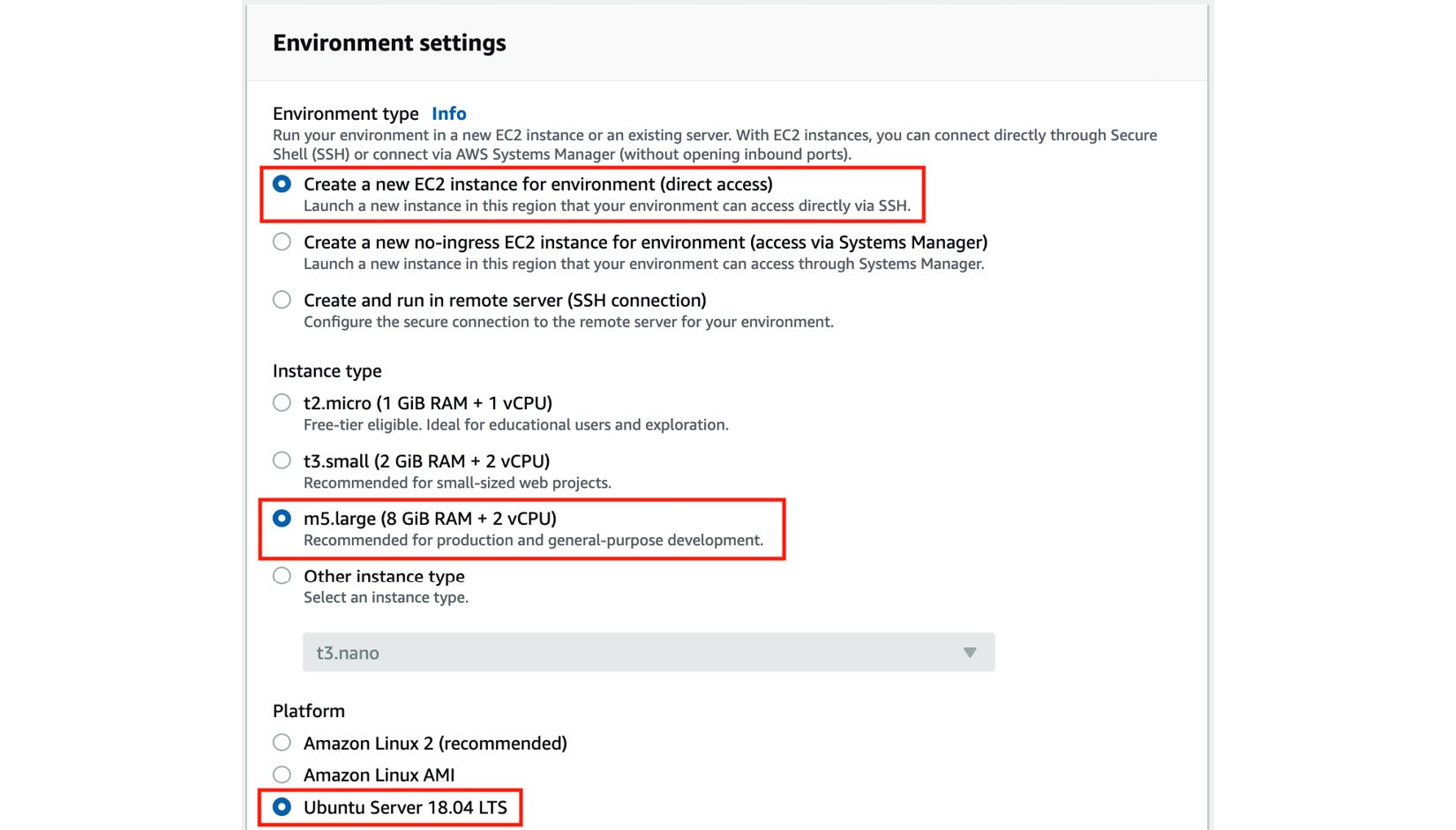
Figure 1.4 – Configuring the Cloud9 environment settings

Here, we can see that there are other options for the instance type. In the meantime, we will stick with m5.large as it should be enough to run the hands-on solutions in this chapter.

5. For the Cost-saving setting option, choose After four hours from the list of drop-down options. This means that the server where the Cloud9 environment is running will automatically shut down after 4 hours of inactivity.
6. Under Network settings (advanced), select the default VPC of the region for the Network (VPC) configuration. It should have a format similar to vpc-abcdefg (default). For the Subnet option, choose the option that has a format similar to subnet-abcdefg | Default in us-west-2a.

Important note

It is recommended that you use the default VPC since the networking configuration is simple. This will help you avoid issues, especially if you’re just getting started with VPCs. If you encounter any VPC-related issues when launching a Cloud9 instance, you may need to check if the selected subnet has been configured with internet access via the route table configuration in the VPC console. You may retry launching the instance using another subnet or by using a new VPC altogether. If you are planning on creating a new VPC, navigate to https://go.aws/3sRSigt and create a VPC with a Single Public Subnet. If none of these options work, you may try launching the Cloud9 instance in another region. We’ll discuss Virtual Private Cloud (VPC) networks in detail in Chapter 9, Security, Governance, and Compliance Strategies.

7. Click Next Step.
8. On the review page, click Create environment. This should redirect you to the Cloud9 environment, which should take a minute or so to load. The Cloud9 IDE is shown in the following screenshot. This is where we can write our code and run the scripts and commands needed to work on some of the hands-on solutions in this book:

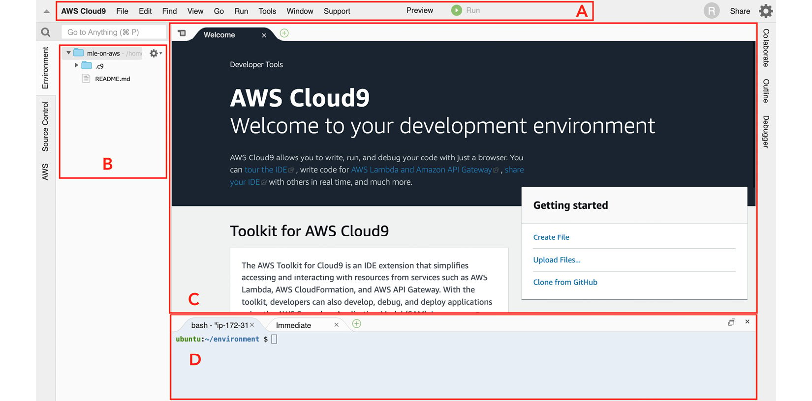
Figure 1.5 – AWS Cloud9 interface

Using this IDE is fairly straightforward as it looks very similar to code editors such as Visual Studio Code and Sublime Text. As shown in the preceding screenshot, we can find the menu bar at the top (A). The file tree can be found on the left-hand side (B). The editor covers a major portion of the screen in the middle (C). Lastly, we can find the terminal at the bottom (D).

Important note

If this is your first time using AWS Cloud9, here is a 4-minute introduction video from AWS to help you get started: https://www.youtube.com/watch?v=JDHZOGMMkj8.

Now that we have our Cloud9 environment ready, it is time we configure it with a larger storage space.

Increasing Cloud9’s storage

When a Cloud9 instance is created, the attached volume only starts with 10GB of disk space. Given that we will be installing different libraries and frameworks while running ML experiments in this instance, we will need more than 10GB of disk space. We will resize the volume programmatically using the boto3 library.

Important note

If this is your first time using the boto3 library, it is the AWS SDK for Python, which gives us a way to programmatically manage the different AWS resources in our AWS accounts. It is a service-level SDK that helps us list, create, update, and delete AWS resources such as EC2 instances, S3 buckets, and EBS volumes.

Follow these steps to download and run some scripts to increase the volume disk space from 10GB to 120GB:

1. In the terminal of our Cloud9 environment (right after the $ sign at the bottom of the screen), run the following bash command:

   wget -O resize_and_reboot.py https://bit.ly/3ea96tW

This will download the script file located at https://bit.ly/3ea96tW. Here, we are simply using a URL shortener, which would map the shortened link to https://raw.githubusercontent.com/PacktPublishing/Machine-Learning-Engineering-on-AWS/main/chapter01/resize_and_reboot.py.

Important note

Note that we are using the big O flag instead of a small o or a zero (0) when using the wget command.

2. What’s inside the file we just downloaded? Let’s quickly inspect the file before we run the script. Double-click the resize_and_reboot.py file in the file tree (located on the left-hand side of the screen) to open the Python script file in the editor pane. As shown in the following screenshot, the resize_and_reboot.py script has three major sections. The first block of code focuses on importing the prerequisites needed to run the script. The second block of code focuses on resizing the volume of a selected EC2 instance using the boto3 library. It makes use of the describe_volumes() method to get the volume ID of the current instance, and then makes use of the modify_volume() method to update the volume size to 120GB. The last section involves a single line of code that simply reboots the EC2 instance. This line of code uses the os.system() method to run the sudo reboot shell command:

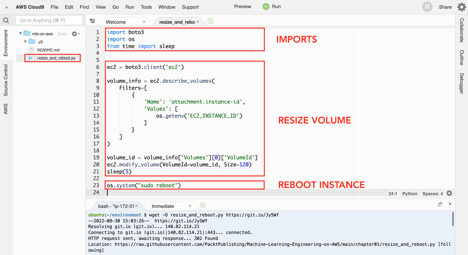
Figure 1.6 – The resize_and_reboot.py script file

You can find the resize_and_reboot.py script file in this book’s GitHub repository: https://github.com/PacktPublishing/Machine-Learning-Engineering-on-AWS/blob/main/chapter01/resize_and_reboot.py. Note that for this script to work, the EC2_INSTANCE_ID environment variable must be set to select the correct target instance. We’ll set this environment variable a few steps from now before we run the resize_and_reboot.py script.

3. Next, run the following command in the terminal:

   python3 -m pip install --user --upgrade boto3

This will upgrade the version of boto3 using pip.

Important note

If this is your first time using pip, it is the package installer for Python. It makes it convenient to install different packages and libraries using the command line.

You may use python3 -m pip show boto3 to check the version you are using. This book assumes that you are using version 1.20.26 or later.

4. The remaining statements focus on getting the Cloud9 environment’s instance_id from the instance metadata service and storing this value in the EC2_INSTANCE_ID variable. Let’s run the following in the terminal:

   TARGET_METADATA_URL=http://169.254.169.254/latest/meta-data/instance-id
   export EC2_INSTANCE_ID=$(curl -s $TARGET_METADATA_URL)
   echo $EC2_INSTANCE_ID

This should give us an EC2 instance ID with a format similar to i-01234567890abcdef.

5. Now that we have the EC2_INSTANCE_ID environment variable set with the appropriate value, we can run the following command:

   python3 resize_and_reboot.py

This will run the Python script we downloaded earlier using the wget command. After performing the volume resize operation using boto3, the script will reboot the instance. You should see a Reconnecting… notification at the top of the page while the Cloud9 environment’s EC2 instance is being restarted.

Important note

Feel free to run the lsblk command after the instance has been restarted. This should help you verify that the volume of the Cloud9 environment instance has been resized to 120GB.

Now that we have successfully resized the volume to 120GB, we should be able to work on the next set of solutions without having to worry about disk space issues inside our Cloud9 environment.

Installing the Python prerequisites

Follow these steps to install and update several Python packages inside the Cloud9 environment:

1. In the terminal of our Cloud9 environment (right after the $ sign at the bottom of the screen), run the following commands to update pip, setuptools, and wheel:

   python3 -m pip install -U pip
   python3 -m pip install -U setuptools wheel

Upgrading these versions will help us make sure that the other installation steps work smoothly. This book assumes that you are using the following versions or later: pip – 21.3.1, setuptools – 59.6.0, and wheel – 0.37.1.

Important note

To check the versions, you may use the python3 -m pip show <package> command in the terminal. Simply replace <package> with the name of the package. An example of this would be python3 -m pip show wheel. If you want to install a specific version of a package, you may use python3 -m pip install -U <package>==<version>. For example, if you want to install wheel version 0.37.1, you can run python3 -m pip install -U wheel==0.37.1.

2. Next, install ipython by running the following command. IPython provides a lot of handy utilities that help professionals use Python interactively. We will see how easy it is to use IPython later in the Performing your first AutoGluon AutoML experiment section:

   python3 -m pip install ipython

This book assumes that you are using ipython – 7.16.2 or later.

3. Now, let’s install ctgan. CTGAN allows us to utilize Generative Adversarial Network (GAN) deep learning models to generate synthetic datasets. We will discuss this shortly in the Generating a synthetic dataset using a deep learning model section, after we have installed the Python prerequisites:

   python3 -m pip install ctgan==0.5.0

This book assumes that you are using ctgan – 0.5.0.

Important note

This step may take around 5 to 10 minutes to complete. While waiting, let’s talk about what CTGAN is. CTGAN is an open source library that uses deep learning to learn about the properties of an existing dataset and generates a new dataset with columns, values, and properties similar to the original dataset. For more information, feel free to check its GitHub page here: https://github.com/sdv-dev/CTGAN.

4. Finally, install pandas_profiling by running the following command. This allows us to easily generate a profile report for our dataset, which will help us with our exploratory data analysis (EDA) work. We will see this in action in the Exploratory data analysis section, after we have generated the synthetic dataset:

   python3 -m pip install pandas_profiling

This book assumes that you are using pandas_profiling – 3.1.0 or later.

Now that we have finished installing the Python prerequisites, we can start generating a realistic synthetic dataset using a deep learning model!

In this chapter, we will build multiple ML models that will predict whether a hotel booking will be cancelled or not based on the information available. Hotel cancellations cause a lot of issues for hotel owners and managers, so trying to predict which reservations will be cancelled is a good use of our ML skills.

Before we start with our ML experiments, we will need a dataset that can be used when training our ML models. We will generate a realistic synthetic dataset similar to the Hotel booking demands dataset from Nuno Antonio, Ana de Almeida, and Luis Nunes.

The synthetic dataset will have a total of 21 columns. Here are some of the columns:

• is_cancelled: Indicates whether the hotel booking was cancelled or not
• lead_time: [arrival date] – [booking date]
• adr: Average daily rate
• adults: Number of adults
• days_in_waiting_list: Number of days a booking stayed on the waiting list before getting confirmed
• assigned_room_type: The type of room that was assigned
• total_of_special_requests: The total number of special requests made by the customer

We will not discuss each of the fields in detail, but this should help us understand what data is available for us to use. For more information, you can find the original version of this dataset at https://www.kaggle.com/jessemostipak/hotel-booking-demand and https://www.sciencedirect.com/science/article/pii/S2352340918315191.

Generating a synthetic dataset using a deep learning model

One of the cool applications of ML would be having a deep learning model “absorb” the properties of an existing dataset and generate a new dataset with a similar set of fields and properties. We will use a pre-trained Generative Adversarial Network (GAN) model to generate the synthetic dataset.

Important note

Generative modeling involves learning patterns from the values of an input dataset, which are then used to generate a new dataset with a similar set of values. GANs are popular when it comes to generative modeling. For example, research papers have focused on how GANs can be used to generate “deepfakes,” where realistic images of humans are generated from a source dataset.

Generating and using a synthetic dataset has a lot of benefits, including the following:

• The ability to generate a much larger dataset than the original dataset that was used to train the model
• The ability to anonymize any sensitive information in the original dataset
• Being able to have a cleaner version of the dataset after data generation

That said, let’s start generating the synthetic dataset by running the following commands in the terminal of our Cloud9 environment (right after the $ sign at the bottom of the screen):

1. Continuing from where we left off in the Installing the Python prerequisites section, run the following command to create an empty directory named tmp in the current working directory:

   mkdir -p tmp

Note that this is different from the /tmp directory.

2. Next, let’s download the utils.py file using the wget command:

   wget -O utils.py https://bit.ly/3CN4owx

The utils.py file contains the block() function, which will help us read and troubleshoot the logs generated by our scripts.

3. Run the following command to download the pre-built GAN model into the Cloud9 environment:

   wget -O hotel_bookings.gan.pkl https://bit.ly/3CHNQFT

Here, we have a serialized pickle file that contains the properties of the deep learning model.

Important note

There are a variety of ways to save and load ML models. One of the options would be to use the Pickle module to serialize a Python object and store it in a file. This file can later be loaded and deserialized back to a Python object with a similar set of properties.

4. Create an empty data_generator.py script file using the touch command:

   touch data_generator.py

Important note

Before proceeding, make sure that the data_generator.py, hotel_bookings.gan.pkl, and utils.py files are in the same directory so that the synthetic data generator script works.

5. Double-click the data_generator.py file in the file tree (located on the left-hand side of the Cloud9 environment) to open the empty Python script file in the editor pane.
6. Add the following lines of code to import the prerequisites needed to run the script:

   from ctgan import CTGANSynthesizer
   from pandas_profiling import ProfileReport
   from utils import block, debug

7. Next, let’s add the following lines of code to load the pre-trained GAN model:

   with block('LOAD CTGAN'):
       pkl = './hotel_bookings.gan.pkl'
       gan = CTGANSynthesizer.load(pkl)
       print(gan.__dict__)

8. Run the following command in the terminal (right after the $ sign at the bottom of the screen) to test if our initial blocks of code in the script are working as intended:

   python3 data_generator.py

This should give us a set of logs similar to what is shown in the following screenshot:

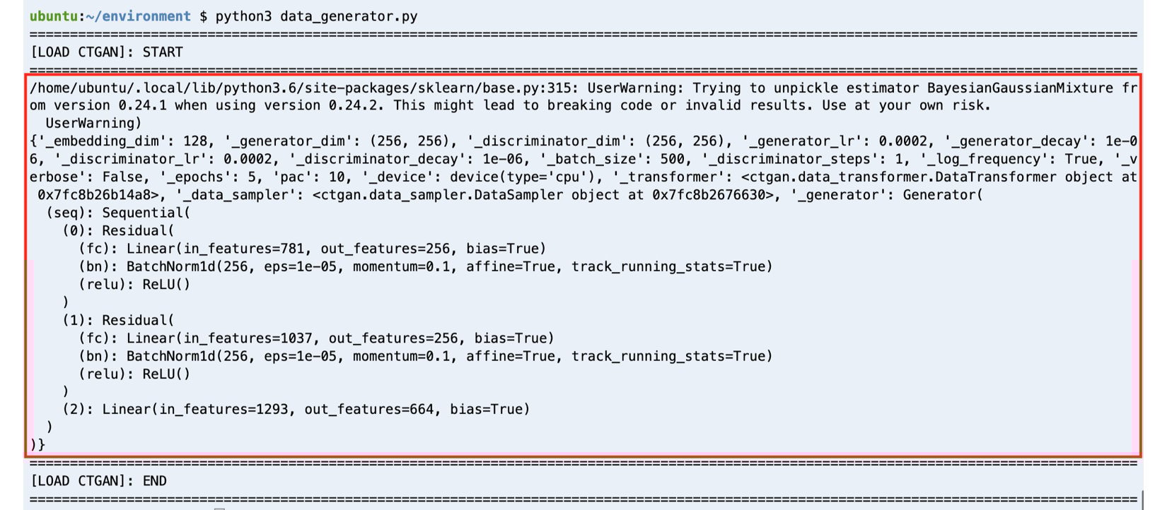
Figure 1.7 – GAN model successfully loaded by the script

Here, we can see that the pre-trained GAN model was loaded successfully using the CTGANSynthesizer.load() method. Here, we can also see what block (from the utils.py file we downloaded earlier) does to improve the readability of our logs. It simply helps mark the start and end of the execution of a block of code so that we can easily debug our scripts.

9. Let’s go back to the editor pane (where we are editing data_generator.py) and add the following lines of code:

   with block('GENERATE SYNTHETIC DATA'):
       synthetic_data = gan.sample(10000)
       print(synthetic_data)

When we run the script later, these lines of code will generate 10000 records and store them inside the synthetic_data variable.

10. Next, let’s add the following block of code, which will save the generated data to a CSV file inside the tmp directory:

    with block('SAVE TO CSV'):
        target_location = "tmp/bookings.all.csv"
        print(target_location)
        synthetic_data.to_csv(
            target_location, 
            index=False
        )

11. Finally, let’s add the following lines of code to complete the script:

    with block('GENERATE PROFILE REPORT'):
        profile = ProfileReport(synthetic_data)
        target_location = "tmp/profile-report.html"
        profile.to_file(target_location)

This block of code will analyze the synthetic dataset and generate a profile report to help us analyze the properties of our dataset.

Important note

You can find a copy of the data_generator.py file here: https://github.com/PacktPublishing/Machine-Learning-Engineering-on-AWS/blob/main/chapter01/data_generator.py.

12. With everything ready, let’s run the following command in the terminal (right after the $ sign at the bottom of the screen):

    python3 data_generator.py

It should take about a minute or so for the script to finish. Running the script should give us a set of logs similar to what is shown in the following screenshot:

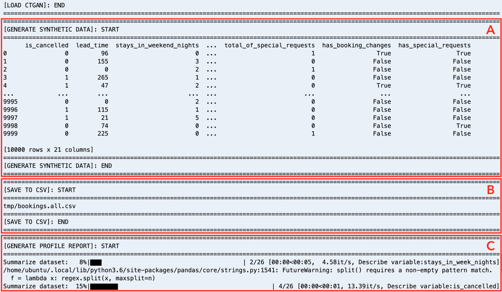
Figure 1.8 – Logs generated by data_generator.py

As we can see, running the data_generator.py script generates multiple blocks of logs, which should make it easy for us to read and debug what’s happening while the script is running. In addition to loading the CTGAN model, the script will generate the synthetic dataset using the deep learning model (A), save the generated data in a CSV file inside the tmp directory (tmp/bookings.all.csv) (B), and generate a profile report using pandas_profiling (C).

Wasn’t that easy? Before proceeding to the next section, feel free to use the file tree (located on the left-hand side of the Cloud9 environment) to check the generated files stored in the tmp directory.

Exploratory data analysis

At this point, we should have a synthetic dataset with 10000 rows. You might be wondering what our data looks like. Does our dataset contain invalid values? Do we have to worry about missing records? We must have a good understanding of our dataset since we may need to clean and process the data first before we do any model training work. EDA is a key step when analyzing datasets before they can be used to train ML models. There are different ways to analyze datasets and generate reports — using pandas_profiling is one of the faster ways to perform EDA.

That said, let’s check the report that was generated by the pandas_profiling Python library. Right-click on tmp/profile-report.html in the file tree (located on the left-hand side of the Cloud9 environment) and then select Preview from the list of options. We should find a report similar to the following:

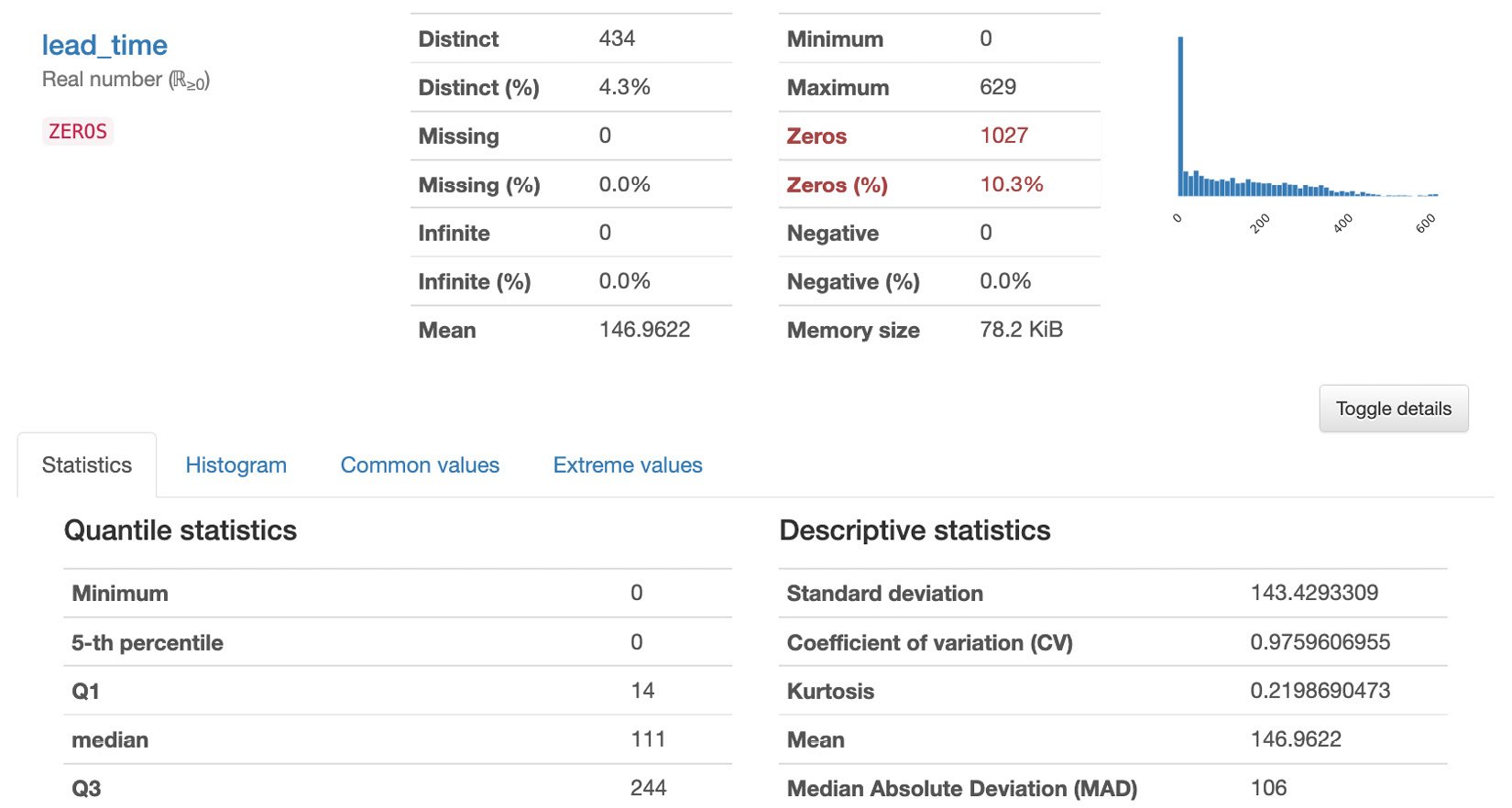
Figure 1.9 – Generated report

The report has multiple sections: Overview, Variables, Interactions, Correlations Missing Values, and Sample. In the Overview section, we can find a quick summary of the dataset statistics and the variable types. This includes the number of variables, number of records (observations), number of missing cells, number of duplicate rows, and other relevant statistics. In the Variables section, we can find the statistics and the distribution of values for each variable (column) in the dataset. In the Interactions and Correlations sections, we can see different patterns and observations regarding the potential relationship of the variables in the dataset. In the Missing values section, we can see if there are columns with missing values that we need to take care of. Finally, in the Sample section, we can see the first 10 and last 10 rows of the dataset.

Feel free to read through the report before proceeding to the next section.

Train-test split

Now that we have finished performing EDA, what do we do next? Assuming that our data is clean and ready for model training, do we just use all of the 10,000 records that were generated to train and build our ML model? Before we train our binary classifier model, we must split our dataset into training and test sets:

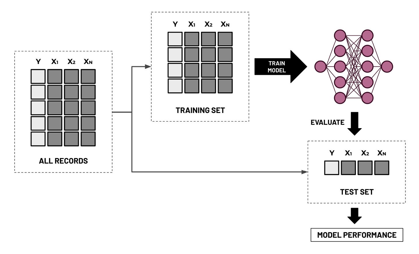
Figure 1.10 – Train-test split

As we can see, the training set is used to build the model and update its parameters during the training phase. The test set is then used to evaluate the final version of the model on data it has not seen before. What’s not shown here is the validation set, which is used to evaluate a model to fine-tune the hyperparameters during the model training phase. In practice, the ratio when dividing the dataset into training, validation, and test sets is generally around 60:20:20, where the training set gets the majority of the records. In this chapter, we will no longer need to divide the training set further into smaller training and validation sets since the AutoML tools and services will automatically do this for us.

Important note

Before proceeding with the hands-on solutions in this section, we must have an idea of what hyperparameters and parameters are. Parameters are the numerical values that a model uses when performing predictions. We can think of model predictions as functions such as y = m * x, where m is a parameter, x is a single predictor variable, and y is the target variable. For example, if we are testing the relationship between cancellations (y) and income (x), then m is the parameter that defines this relationship. If m is positive, cancellations go up as income goes up. If it is negative, cancellations lessen as income increases. On the other hand, hyperparameters are configurable values that are tweaked before the model is trained. These variables affect how our chosen ML models “model” the relationship. Each ML model has its own set of hyperparameters, depending on the algorithm used. These concepts will make more sense once we have looked at a few more examples in Chapter 2, Deep Learning AMIs, and Chapter 3, Deep Learning Containers.

Now, let’s create a script that will help us perform the train-test split:

1. In the terminal of our Cloud9 environment (right after the $ sign at the bottom of the screen), run the following command to create an empty file called train_test_split.py:

   touch train_test_split.py

2. Using the file tree (located on the left-hand side of the Cloud9 environment), double-click the train_test_split.py file to open the file in the editor pane.
3. In the editor pane, add the following lines of code to import the prerequisites to run the script:

   import pandas as pd
   from utils import block, debug
   from sklearn.model_selection import train_test_split

4. Add the following block of code, which will read the contents of a CSV file and store it inside a pandas DataFrame:

   with block('LOAD CSV'):
       generated_df = pd.read_csv('tmp/bookings.all.csv')

5. Next, let’s use the train_test_split() function from scikit-learn to divide the dataset we have generated into a training set and a test set:

   with block('TRAIN-TEST SPLIT'):
       train_df, test_df = train_test_split(
           generated_df, 
           test_size=0.3, 
           random_state=0
       )
       print(train_df)
       print(test_df)

6. Lastly, add the following lines of code to save the training and test sets into their respective CSV files inside the tmp directory:

   with block('SAVE TO CSVs'):
       train_df.to_csv('tmp/bookings.train.csv', 
                       index=False)
       test_df.to_csv('tmp/bookings.test.csv', 
                      index=False)

Important note

You can find a copy of the train_test_split.py file here: https://github.com/PacktPublishing/Machine-Learning-Engineering-on-AWS/blob/main/chapter01/train_test_split.py.

7. Now that we have completed our script file, let’s run the following command in the terminal (right after the $ sign at the bottom of the screen):

   python3 train_test_split.py

This should generate a set of logs similar to what is shown in the following screenshot:

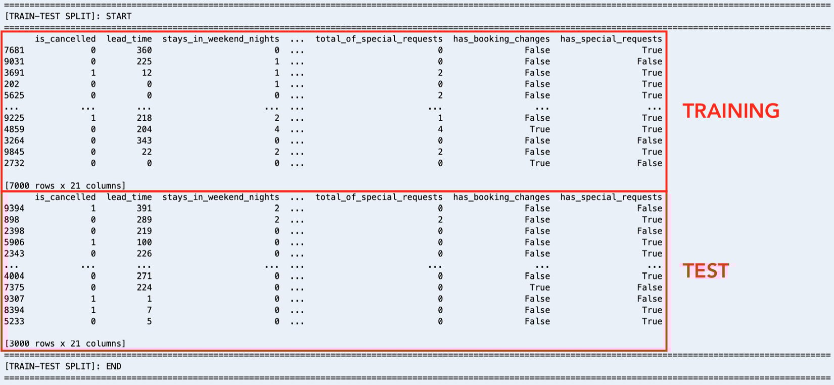
Figure 1.11 – Train-test split logs

Here, we can see that our training dataset contains 7,000 records, while the test set contains 3,000 records.

With this, we can upload our dataset to Amazon S3.

Uploading the dataset to Amazon S3

Amazon S3 is the object storage service for AWS and is where we can store different types of files, such as dataset CSV files and output artifacts. When using the different services of AWS, it is important to note that these services sometimes require the input data and files to be stored in an S3 bucket first or in a resource created using another service.

Uploading the dataset to S3 should be easy. Continuing where we left off in the Train-test split section, we will run the following commands in the terminal:

1. Run the following commands in the terminal. Here, we are going to create a new S3 bucket that will contain the data we will be using in this chapter. Make sure that you replace the value of <INSERT BUCKET NAME HERE> with a bucket name that is globally unique across all AWS users:

   BUCKET_NAME="<INSERT BUCKET NAME HERE>"
   aws s3 mb s3://$BUCKET_NAME

For more information on S3 bucket naming rules, feel free to check out https://docs.aws.amazon.com/AmazonS3/latest/userguide/bucketnamingrules.html.

2. Now that the S3 bucket has been created, let’s upload the training and test datasets using the AWS CLI:

   S3=s3://$BUCKET_NAME/datasets/bookings
   TRAIN=bookings.train.csv
   TEST=bookings.test.csv
   aws s3 cp tmp/bookings.train.csv $S3/$TRAIN
   aws s3 cp tmp/bookings.test.csv $S3/$TEST

Now that everything is ready, we can proceed with the exciting part! It’s about time we perform multiple AutoML experiments using a variety of solutions and services.

Previously, we discussed what hyperparameters are. When training and tuning ML models, it is important for us to know that the performance of an ML model depends on the algorithm, the training data, and the hyperparameter configuration that’s used when training the model. Other input configuration parameters may also affect the performance of the model, but we’ll focus on these three for now. Instead of training a single model, teams build multiple models using a variety of hyperparameter configurations. Changes and tweaks in the hyperparameter configuration affect the performance of a model – some lead to better performance, while others lead to worse performance. It takes time to try out all possible combinations of hyperparameter configurations, especially if the model tuning process is not automated.

These past couple of years, several libraries, frameworks, and services have allowed teams to make the most out of automated machine learning (AutoML) to automate different parts of the ML process. Initially, AutoML tools focused on automating the hyperparameter optimization (HPO) processes to obtain the optimal combination of hyperparameter values. Instead of spending hours (or even days) manually trying different combinations of hyperparameters when running training jobs, we’ll just need to configure, run, and wait for this automated program to help us find the optimal set of hyperparameter values. For years, several tools and libraries that focus on automated hyperparameter optimization were available for ML practitioners for use. After a while, other aspects and processes of the ML workflow were automated and included in the AutoML pipeline.

There are several tools and services available for AutoML and one of the most popular options is AutoGluon. With AutoGluon, we can train multiple models using different algorithms and evaluate them with just a few lines of code:

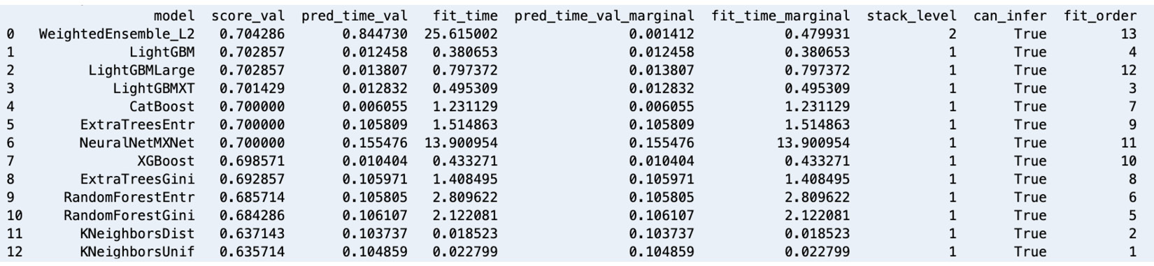
Figure 1.12 – AutoGluon leaderboard – models trained using a variety of algorithms

Similar to what is shown in the preceding screenshot, we can also compare the generated models using a leaderboard. In this chapter, we’ll use AutoGluon with a tabular dataset. However, it is important to note that AutoGluon also supports performing AutoML tasks for text and image data.

Setting up and installing AutoGluon

Before using AutoGluon, we need to install it. It should take a minute or so to complete the installation process:

1. Run the following commands in the terminal to install and update the prerequisites before we install AutoGluon:

   python3 -m pip install -U "mxnet<2.0.0"
   python3 -m pip install numpy
   python3 -m pip install cython
   python3 -m pip install pyOpenSSL --upgrade

This book assumes that you are using the following versions or later: mxnet – 1.9.0, numpy – 1.19.5, and cython – 0.29.26.

2. Next, run the following command to install autogluon:

   python3 -m pip install autogluon

This book assumes that you are using autogluon version 0.3.1 or later.

Important note

This step may take around 5 to 10 minutes to complete. Feel free to grab a cup of coffee or tea!

With AutoGluon installed in our Cloud9 environment, let’s proceed with our first AutoGluon AutoML experiment.

Performing your first AutoGluon AutoML experiment

If you have used scikit-learn or other ML libraries and frameworks before, using AutoGluon should be easy and fairly straightforward since it uses a very similar set of methods, such as fit() and predict(). Follow these steps:

1. To start, run the following command in the terminal:

   ipython

This will open the IPython Read-Eval-Print-Loop (REPL)/interactive shell. We will use this similar to how we use the Python shell.

2. Inside the console, type in (or copy) the following block of code. Make sure that you press Enter after typing the closing parenthesis:

   from autogluon.tabular import (
       TabularDataset,
       TabularPredictor
   )

3. Now, let’s load the synthetic data stored in the bookings.train.csv and bookings.test.csv files into the train_data and test_data variables, respectively, by running the following statements:

   train_loc = 'tmp/bookings.train.csv'
   test_loc = 'tmp/bookings.test.csv'
   train_data = TabularDataset(train_loc)
   test_data = TabularDataset(test_loc)

Since the parent class of AutoGluon, TabularDataset, is a pandas DataFrame, we can use different methods on train_data and test_data such as head(), describe(), memory_usage(), and more.

4. Next, run the following lines of code:

   label = 'is_cancelled'
   save_path = 'tmp'
   tp = TabularPredictor(label=label, path=save_path)
   predictor = tp.fit(train_data)

Here, we specify is_cancelled as the target variable of the AutoML task and the tmp directory as the location where the generated models will be stored. This block of code will use the training data we have provided to train multiple models using different algorithms. AutoGluon will automatically detect that we are dealing with a binary classification problem and generate multiple binary classifier models using a variety of ML algorithms.

Important note

Inside the tmp/models directory, we should find CatBoost, ExtraTreesEntr, and ExtraTreesGini, along with other directories corresponding to the algorithms used in the AutoML task. Each of these directories contains a model.pkl file that contains the serialized model. Why do we have multiple models? Behind the scenes, AutoGluon runs a significant number of training experiments using a variety of algorithms, along with different combinations of hyperparameter values, to produce the “best” model. The “best” model is selected using a certain evaluation metric that helps identify which model performs better than the rest. For example, if the evaluation metric that’s used is accuracy, then a model with an accuracy score of 90% (which gets 9 correct answers every 10 tries) is “better” than a model with an accuracy score of 80% (which gets 8 correct answers every 10 tries). That said, once the models have been generated and evaluated, AutoGluon simply chooses the model with the highest evaluation metric value (for example, accuracy) and tags it as the “best model.”

5. Now that we have our “best model” ready, what do we do next? The next step is for us to evaluate the “best model” using the test dataset. That said, let’s prepare the test dataset for inference by removing the target label:

   y_test = test_data[label]
   test_data_no_label = test_data.drop(columns=[label])

6. With everything ready, let’s use the predict() method to predict the is_cancelled column value of the test dataset provided as the payload:

   y_pred = predictor.predict(test_data_no_label)

7. Now that we have the actual y values (y_test) and the predicted y values (y_pred), let’s quickly check the performance of the trained model by using the evaluate_predictions() method:

   predictor.evaluate_predictions(
       y_true=y_test, 
       y_pred=y_pred, 
       auxiliary_metrics=True
   )

The previous block of code should yield performance metric values similar to the following:

{'accuracy': 0.691...,
 'balanced_accuracy': 0.502...,
 'mcc': 0.0158...,
 'f1': 0.0512...,
 'precision': 0.347...,
 'recall': 0.0276...}

In this step, we compare the actual values with the predicted values for the target column using a variety of formulas that compare how close these values are to each other. Here, the goal of the trained models is to make “the least number of mistakes” as possible over unseen data. Better models generally have better scores for performance metrics such as accuracy, Matthews correlation coefficient (MCC), and F1-score. We won’t go into the details of how model performance metrics work here. Feel free to check out https://bit.ly/3zn2crv for more information.

8. Now that we are done with our quick experiment, let’s exit the IPython shell:

   exit()

There’s more we can do using AutoGluon but this should help us appreciate how easy it is to use AutoGluon for AutoML experiments. There are other methods we can use, such as leaderboard(), get_model_best(), and feature_importance(), so feel free to check out https://auto.gluon.ai/stable/index.html for more information.

When performing ML and ML engineering on AWS, professionals should consider using one or more of the capabilities and features of Amazon SageMaker. If this is your first time learning about SageMaker, it is a fully managed ML service that helps significantly speed up the process of preparing, training, evaluating, and deploying ML models.

If you are wondering what these capabilities are, check out some of the capabilities tagged under ML SERVICES in Figure 1.2 from the How ML engineers can get the most out of AWS section. We will tackle several capabilities of SageMaker as we go through the different chapters of this book. In the meantime, we will start with SageMaker Studio as we will need to set it up first before we work on the SageMaker Canvas and SageMaker Autopilot examples.

Onboarding with SageMaker Studio

SageMaker Studio provides a feature-rich IDE for ML practitioners. One of the great things about SageMaker Studio is its tight integration with the other capabilities of SageMaker, which allows us to manage different SageMaker resources by just using the interface.

For us to have a good idea of what it looks like and how it works, let’s proceed with setting up and configuring SageMaker Studio:

1. In the search bar of the AWS console, type sagemaker studio. Select SageMaker Studio under Features.
2. Choose Standard setup, as shown in the following screenshot:

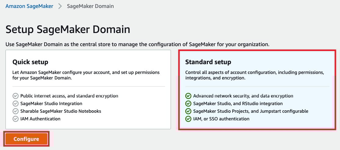
Figure 1.13 – Setup SageMaker Domain

As we can see, Standard setup should give us more configuration options to tweak over Quick setup. Before clicking the Configure button, make sure that you are using the same region where the S3 bucket and training and test datasets are located.

3. Under Authentication, select AWS Identity and Access Management (IAM). For the default execution role under Permission, choose Create a new role. Choose Any S3 bucket. Then, click Create role.
4. Under Network and Storage Section, select the default VPC and choose a subnet (for example, us-west-2a), similar to what is shown in the following screenshot:

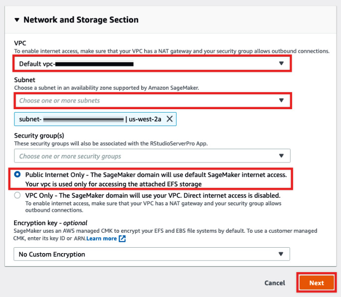
Figure 1.14 – Network and Storage Section

Here, we have also configured the SageMaker Domain to use the default SageMaker internet access by selecting Public Internet Only. Under Encryption key, we leave this unchanged by choosing No Custom Encryption. Review the configuration and then click Next.

Important note

Note that for production environments, the security configuration specified in the last few steps needs to be reviewed and upgraded further. In the meantime, this should do the trick since we’re dealing with a sample dataset. We will discuss how to secure environments in detail in Chapter 9, Security, Governance, and Compliance Strategies.

5. Under Studio settings, leave everything as-is and click Next.
6. Similarly, under General settings | RStudio Workbench, click Submit.

Once you have completed these steps, you should see the Preparing SageMaker Domain loading message. This step should take around 3 to 5 minutes to complete. Once complete, you should see a notification stating The SageMaker Domain is ready.

Adding a user to an existing SageMaker Domain

Now that our SageMaker Domain is ready, let’s create a user. Creating a user is straightforward. So, let’s begin:

1. On the SageMaker Domain/Control Panel page, click Add user.
2. Specify the name of the user under Name. Under Default execution role, select the execution role that you created in the previous step. Click Next.
3. Under Studio settings | SageMaker Projects and JumpStart, click Next.
4. Under RStudio settings | Rstudio Workbench, click Submit.

This should do the trick for now. In Chapter 9, Security, Governance, and Compliance Strategies, we will review how we can improve the configuration here to improve the security of our environment.

Before we proceed with using the more comprehensive set of SageMaker capabilities to perform ML experiments and deployments, let’s start by building a model using SageMaker Canvas. One of the great things about SageMaker Canvas is that no coding work is needed to build models and use them to perform predictions. Of course, SageMaker Autopilot would have a more powerful and flexible set of features, but SageMaker Canvas should help business analysts, data scientists, and junior ML engineers understand the ML process and get started building models right away.

Since our dataset has already been uploaded to the S3 bucket, we can start building and training our first SageMaker Canvas model:

1. On the SageMaker Domain/Control Panel page, locate the row of the user we just created and click Launch app. Choose Canvas from the list of options available in the drop-down menu, as shown in the following screenshot:

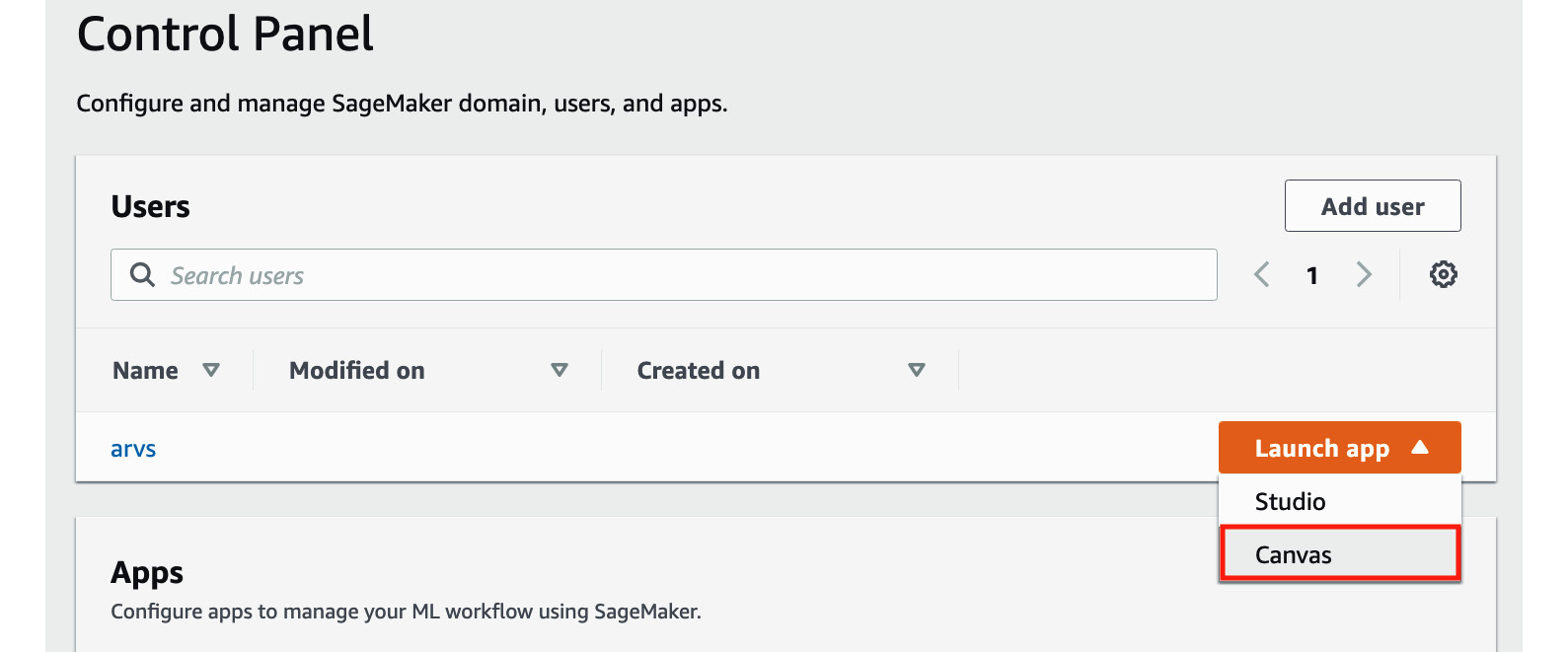
Figure 1.15 – Launching SageMaker Canvas

As we can see, we can launch SageMaker Canvas from the SageMaker Domain/Control Panel page. We can launch SageMaker Studio here as well, which we’ll do later in this chapter.

2. Click New model:

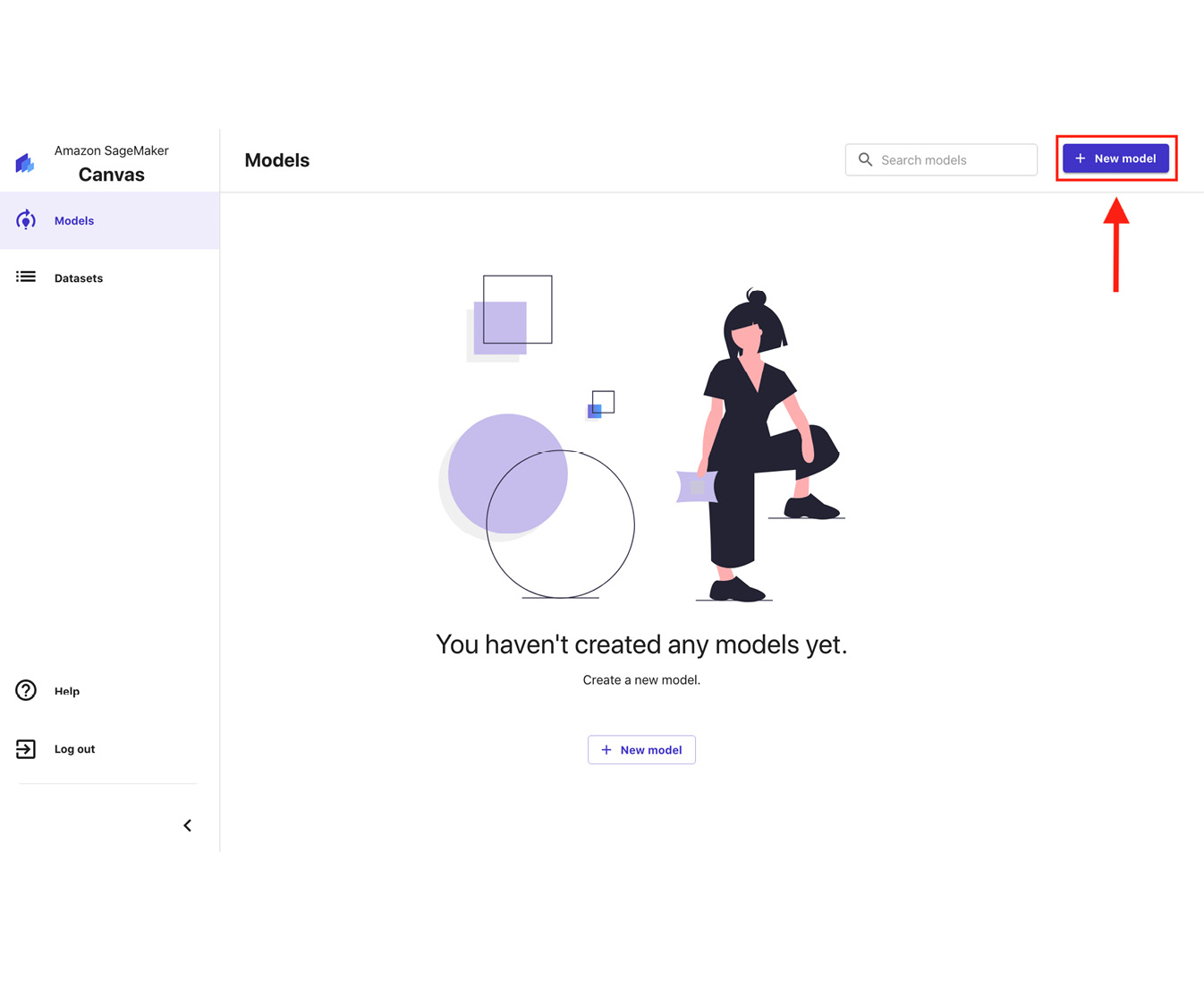
Figure 1.16 – The SageMaker Canvas Models page

Here, we have the SageMaker Canvas Models page, which should list the models we have trained. Since we have not trained anything yet, we should see the You haven’t created any models yet message.

3. In the Create new model popup window, specify the name of the model (for example, first-model) and click Create.
4. When you see the Getting Started guide window, click Skip intro.
5. Click Import data to canvas. Locate the S3 bucket we created earlier in the Uploading the dataset to S3 section. After that, locate the booking.train.csv and booking.test.csv files inside the Amazon S3/<S3 BUCKET>/datasets/bookings folder of the S3 bucket.

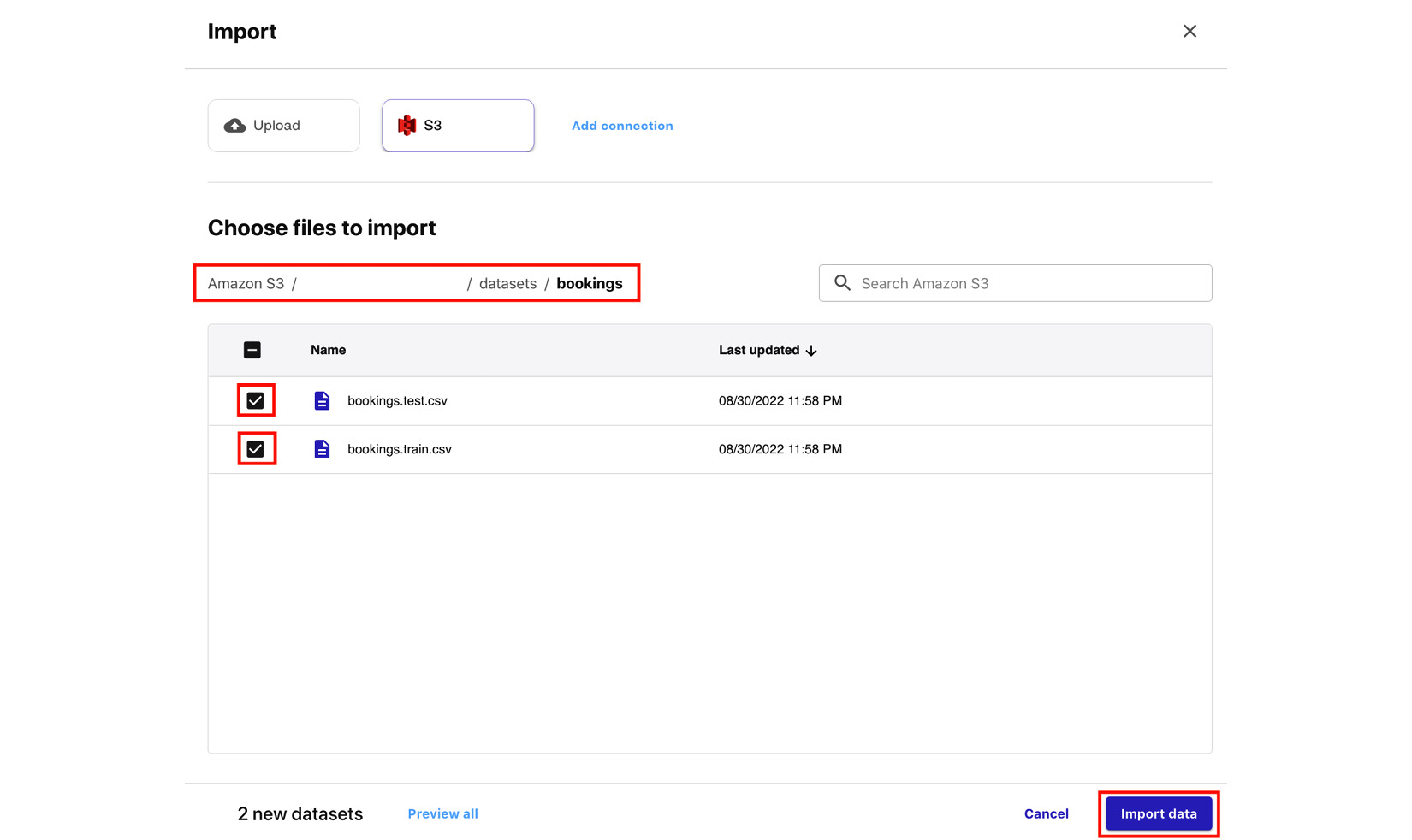
Figure 1.17 – Choose files to import

Select the necessary CSV files, as shown in the preceding screenshot, and click Import data.

Important note

Note that you may have a hard time locating the S3 bucket we created in the Uploading the dataset to S3 section if you have a significant number of S3 buckets in your account. Feel free to use the search box (with the Search Amazon S3 placeholder) located on the right-hand side, just above the table that lists the different S3 buckets and resources.

6. Once the files have been imported, click the radio button of the row that contains bookings.train.csv. Click Select dataset.
7. In the Build tab, click and open the Target column drop-down under Select a column to predict. Select is_cancelled from the list of drop-down options for the Target column field.
8. Next, click Preview model (under the Quick build button), as highlighted in the following screenshot:

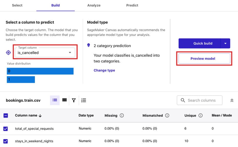
Figure 1.18 – The Build tab

After a few minutes, we should get an estimated accuracy of around 70%. Note that you might get a different set of numbers in this step.

9. Click Quick build and wait for the model to be ready.

Important note

This step may take up to 15 minutes to complete. While waiting, let’s quickly discuss the difference between Quick build and Standard build. Quick build uses fewer records for training and generally lasts around 2 to 15 minutes, while Standard build lasts much longer – generally around 2 to 4 hours. It is important to note that models that are trained using Quick build can’t be shared with other data scientists or ML engineers in SageMaker Studio. On the other hand, models trained using Standard build can be shared after the build has been completed.

10. Once the results are available, you may open the Scoring tab by clicking the tab highlighted in the following screenshot:

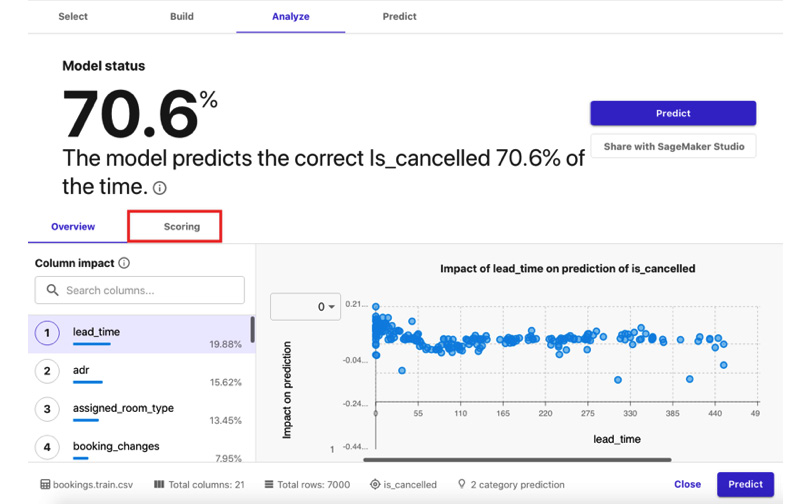
Figure 1.19 – The Analyze tab

We should see a quick chart showing the number of records that were used to analyze the model, along with the number of correct versus incorrect predictions the model has made.

Important note

At this point, we have built an ML model that we can use to predict whether a booking will be cancelled or not. Since the accuracy score in this example is only around 70%, we’re expecting the model to get about 7 correct answers every 10 tries. In Chapter 11, Machine Learning Pipelines with SageMaker Pipelines, we will train an improved version of this model with an accuracy score of around 88%.

11. Once we are done checking the different numbers and charts in the Analyze tab, we can proceed by clicking the Predict button.
12. Click Select dataset. Under Select dataset for predictions, choose bookings.test.csv and click Generate predictions.
13. Once the Status column value is set to Ready, hover over the Status column of the row, click the 3 dots (which will appear after hovering over the row), and then select Preview from the list of options:

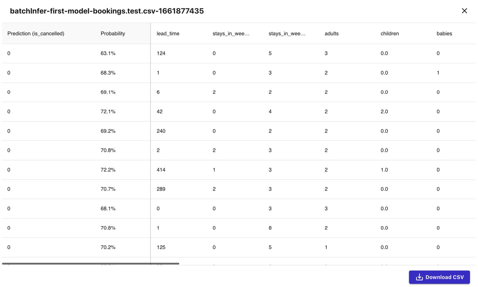
Figure 1.20 – Batch prediction results

We should see a table of values, similar to what is shown in the preceding screenshot. In the first column, we should have the predicted values for the is_cancelled field for each of the rows of our test dataset. In the second column, we should find the probability of the prediction being correct.

Important note

Note that we can also perform a single prediction by using the interface provided after clicking Single prediction under Predict target values.

14. Finally, let’s log out of our session. Click the Account icon in the left sidebar and select the Log out option.

Important note

Make sure that you always log out of the current session after using SageMaker Canvas to avoid any unexpected charges. For more information, go to https://docs.aws.amazon.com/sagemaker/latest/dg/canvas-log-out.html.

Wasn’t that easy? Now that we have a good idea of how to use SageMaker Canvas, let’s run an AutoML experiment using SageMaker Autopilot.

SageMaker Autopilot allows ML practitioners to build high-quality ML models without having to write a single line of code. Of course, it is possible to programmatically configure, run, and manage SageMaker Autopilot experiments using the SageMaker Python SDK, but we will focus on using the SageMaker Studio interface to run the AutoML experiment. Before jumping into configuring our first Autopilot experiment, let’s see what happens behind the scenes:

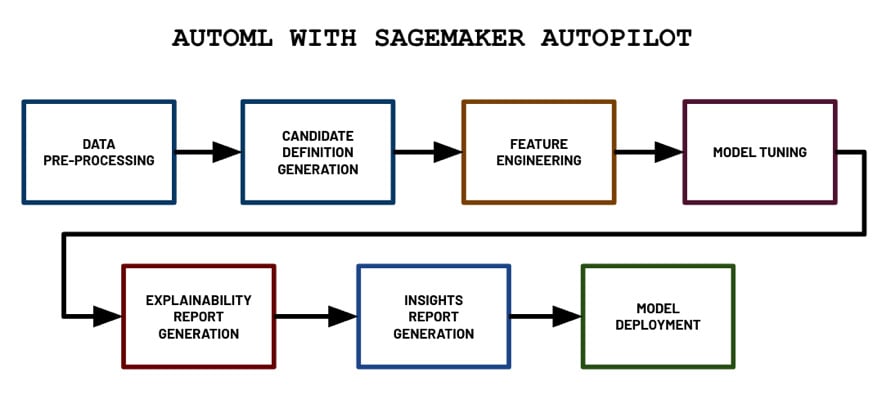
Figure 1.21 – AutoML with SageMaker Autopilot

In the preceding diagram, we can see the different steps that are performed by SageMaker Autopilot when we run the AutoML experiment. It starts with the data pre-processing step and proceeds with the generation of candidate models (pipeline and algorithm pair) step. Then, it continues to perform the feature engineering and model tuning steps, which would yield multiple trained models from different model families, hyperparameter values, and model performance metric values. The generated model with the best performance metric values is tagged as the “best model” by the Autopilot job. Next, two reports are generated: the explainability report and the insights report. Finally, the model is deployed to an inference endpoint.

Let’s dive a bit deeper into what is happening in each step:

• Data pre-processing: Data is cleaned automatically and missing values are automatically imputed.
• Candidate definition generation: Multiple “candidate definitions” (composed of a data processing job and a training job) are generated, all of which will be used on the dataset.
• Feature engineering: Here, data transformations are applied to perform automated feature engineering.
• Model tuning: The Automatic Model Tuning (hyperparameter tuning) capability of SageMaker is used to generate multiple models using a variety of hyperparameter configuration values to find the “best model.”
• Explainability report generation: The model explainability report, which makes use of SHAP values to help explain the behavior of the generated model, is generated using tools provided by SageMaker Clarify (another capability of SageMaker focused on AI fairness and explainability). We’ll dive a bit deeper into this topic later in Chapter 9, Security, Governance, and Compliance Strategies.
• Insights report generation: The insights report, which includes data insights such as scalar metrics, which help us understand our dataset better, is generated.
• Model deployment: The best model is deployed to a dedicated inference endpoint. Here, the value of the objective metric is used to determine which is the best model out of all the models trained during the model tuning step.

Important note

If you are wondering if AutoML solutions would fully “replace” data scientists, then a quick answer to your question would be “no” or “not anytime soon.” There are specific areas of the ML process that require domain knowledge to be available to data scientists. AutoML solutions help provide a good starting point that data scientists and ML practitioners can build on top of. For example, white box AutoML solutions such as SageMaker Autopilot can generate scripts and notebooks that can be modified by data scientists and ML practitioners to produce custom and complex data processing, experiment, and deployment flows and pipelines.

Now that we have a better idea of what happens during an Autopilot experiment, let’s run our first Autopilot experiment:

1. On the Control Panel page, click the Launch app drop-down menu and choose Studio from the list of drop-down options, as shown in the following screenshot:

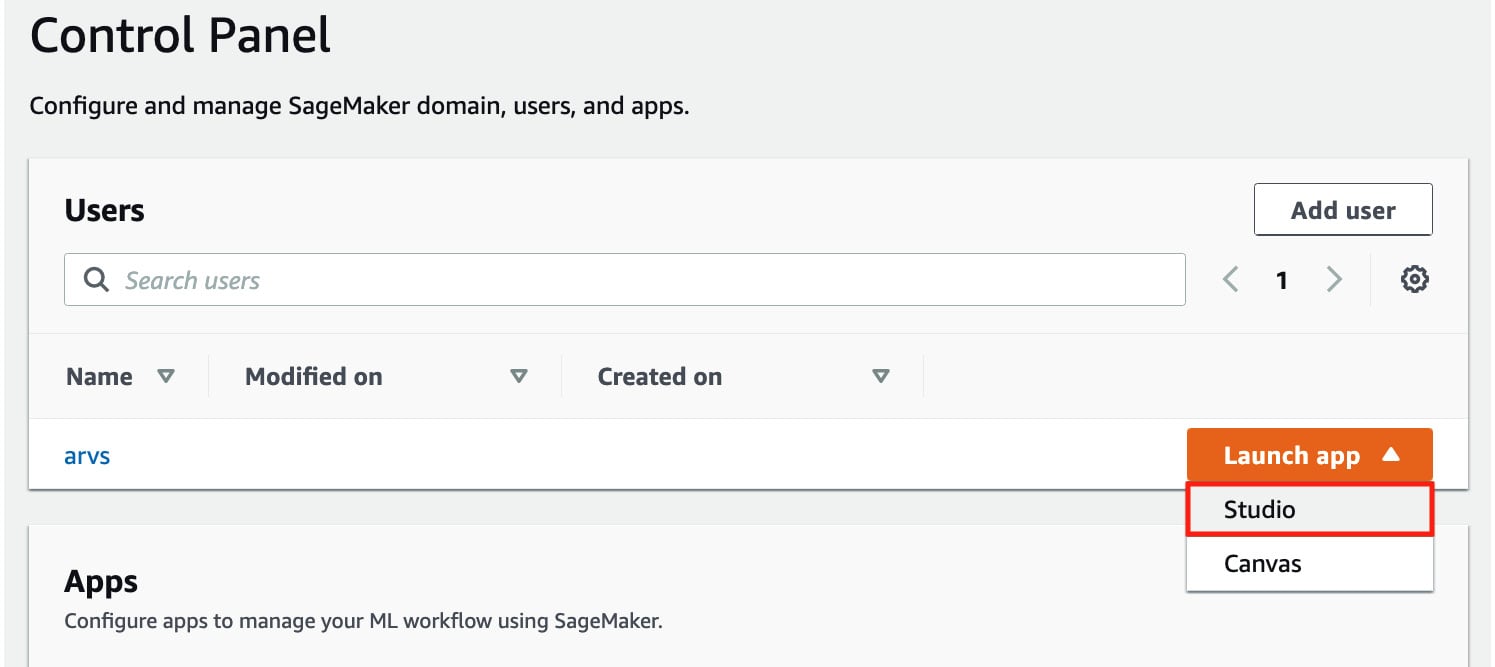
Figure 1.22 – Opening SageMaker Studio

Note that it may take around 5 minutes for SageMaker Studio to load if this is your first time opening it.

Important note

AWS releases updates and upgrades for SageMaker Studio regularly. To ensure that you are using the latest version, make sure that you shut down and update SageMaker Studio and Studio Apps. For more information, go to https://docs.aws.amazon.com/sagemaker/latest/dg/studio-tasks-update.html.

2. Open the File menu and click Experiment under the New submenu:

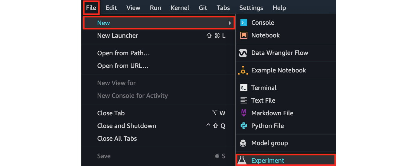
Figure 1.23 – Using the File menu to create a new experiment

Here, we have multiple options under the New submenu. We will explore the other options throughout this book.

In the next set of steps, we will configure the Autopilot experiment, similar to what is shown in the following screenshot:

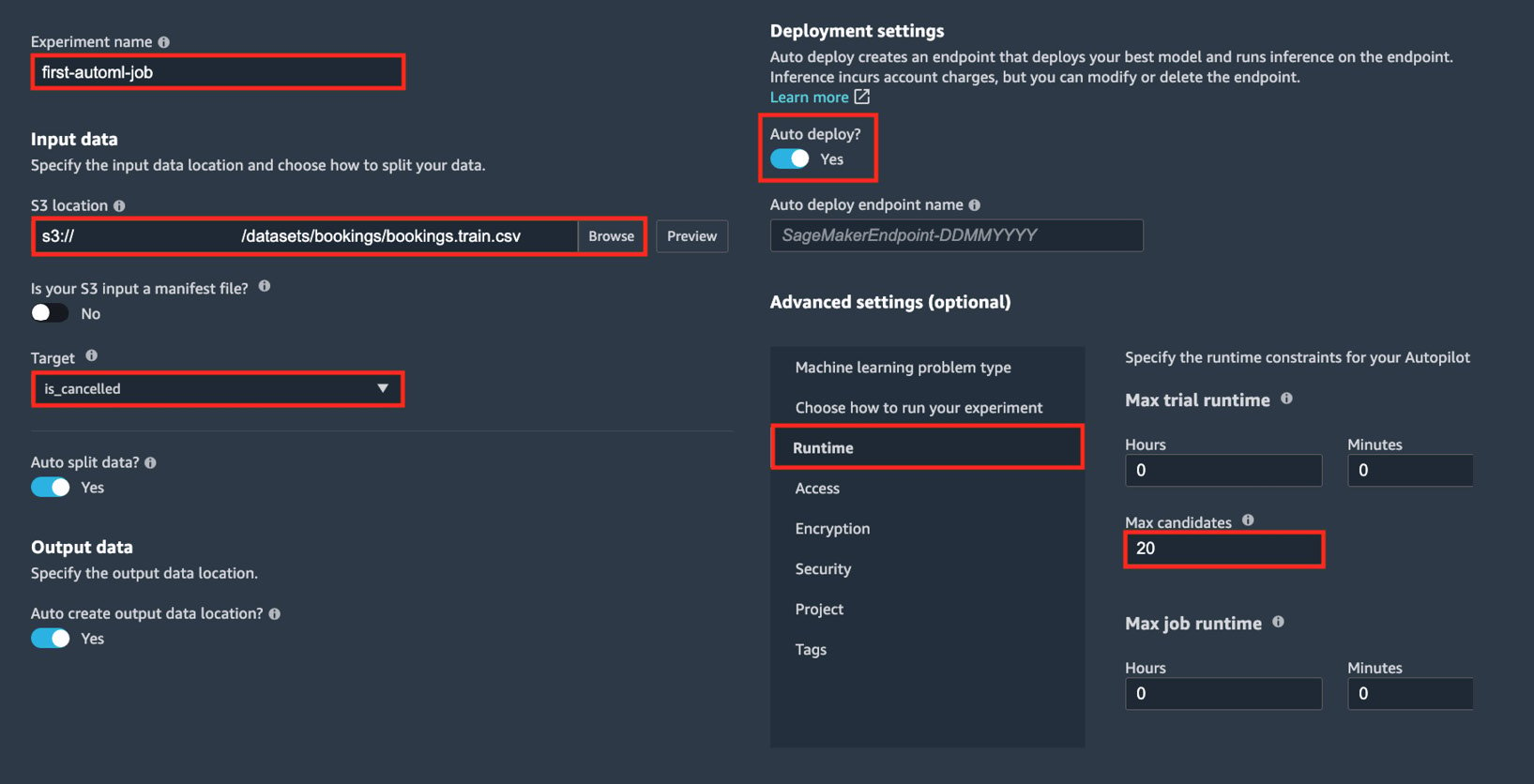
Figure 1.24 – Configuring the Autopilot experiment

Here, we can see the different configuration options that are available before running the Autopilot experiment. Note that the actual Autopilot experiment settings form only has a single column instead of two.

1. Specify the Experiment name value (for example, first-automl-job).
2. Under Input data, locate and select the bookings.train.csv we uploaded earlier by clicking Browse.
3. In the Target drop-down menu, choose is_cancelled. Click Next: Training method.
4. Leave everything else as is, and then click Next: Deployment and advanced settings.
5. Make sure that the Auto deploy? configuration is set to Yes.

Important note

You may opt to set the Auto deploy configuration to No instead so that an inference endpoint will not be created by the Autopilot job. If you have set this to Yes make sure that you delete the inference endpoint if you are not using it.

6. Under Advanced Settings (optional) > Runtime, set Max Candidates to 20 (or alternatively, setting both Max trial runtime Minutes and Max job runtime Minutes to 20). Click Next: Review and create.

Important note

Setting the value for Max Candidates to 20 means that Autopilot will train and consider only 20 candidate models for this Autopilot job. Of course, we can set this to a higher number, which would increase the chance of finding a candidate with a higher evaluation metric score (for example, a model that performs better). However, this would mean that it would take longer for Autopilot to run since we’ll be running more training jobs. Since we are just trying out this capability, we should be fine setting Max Candidates to 20 in the meantime.

7. Review all the configuration parameters we have set in the previous steps and click Create experiment. When asked if you want to auto-deploy the best model, click Confirm. Once the AutoML job has started, we should see a loading screen similar to the following:

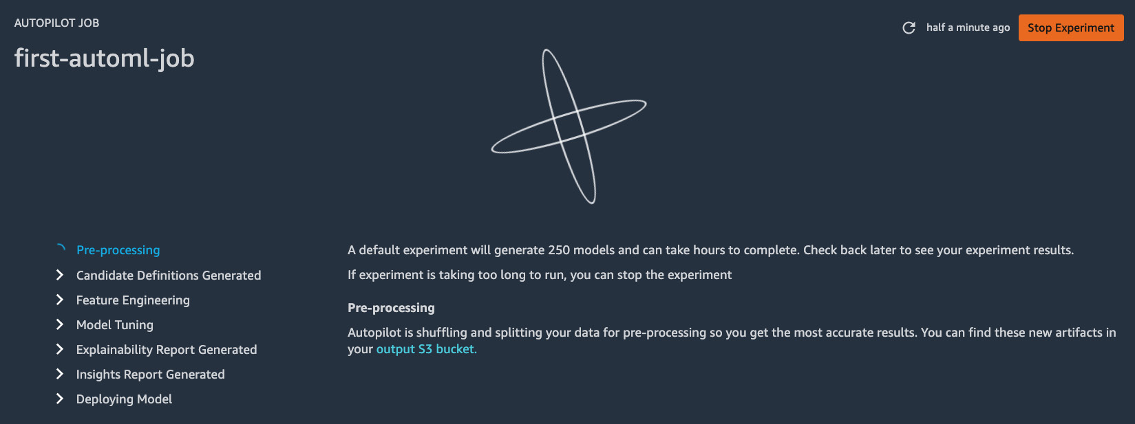
Figure 1.25 – Waiting for the AutoML job to complete

Here, we can see that the Autopilot job involves the following steps:

1. Pre-processing
2. Candidate Definitions Generated
3. Feature Engineering
4. Model Tuning
5. Explainability Report Generated
6. Insights Report Generated
7. Deploying Model

If we have set the Auto deploy configuration to Yes, the best model is deployed automatically into an inference endpoint that will run 24/7.

Important note

This step may take around 30 minutes to 1 hour to complete. Feel free to get a cup of coffee or tea!

After about an hour, we should see a list of trials, along with several models that have been generated by multiple training jobs, as shown in the following screenshot:

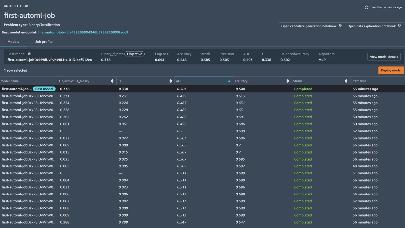
Figure 1.26 – Autopilot job results

We should also see two buttons on the top right-hand side of the page: Open candidate generation notebook and Open data exploration notebook. Since these two notebooks are generated early in the process, we may see the buttons appear about 10 to 15 minutes after the experiment started.

8. Click the Open candidate generation notebook and Open data exploration notebook buttons to open the notebooks that were generated by SageMaker Autopilot:

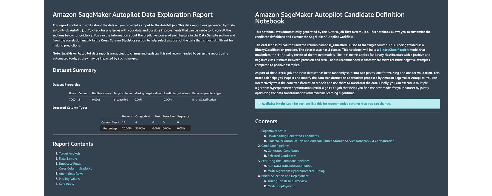
Figure 1.27 – The Data Exploration Report (left) and the Candidate Definition Notebook (right)

Here, we can see the Data Exploration Report on the left-hand side and the Candidate Definition Notebook on the right. The Data Exploration Report helps data scientists and ML engineers identify issues in the given dataset. It contains a column analysis report that shows the percentage of missing values, along with some count statistics and descriptive statistics. On the other hand, the Candidate Definition Notebook contains the suggested ML algorithm, along with the prescribed hyperparameter ranges. In addition to these, it contains the recommended pre-processing steps before the training step starts.

The great thing about these generated notebooks is that we can modify certain sections of these notebooks as needed. This makes SageMaker Autopilot easy for beginners to use while still allowing intermediate users to customize certain parts of the AutoML process.

Important note

If you want to know more about SageMaker Autopilot, including the output artifacts generated by the AutoML experiment, check out Chapter 6, SageMaker Training and Debugging Solutions, of the book Machine Learning with Amazon SageMaker Cookbook. You should find several recipes there that focus on programmatically running and managing an Autopilot experiment using the SageMaker Python SDK.

9. Navigate back to the tab containing the results of the Autopilot job. Right-click on the row with the Best Model tag and choose Open in model details from the options in the context menu. This should open a page similar to what is shown in the following screenshot:

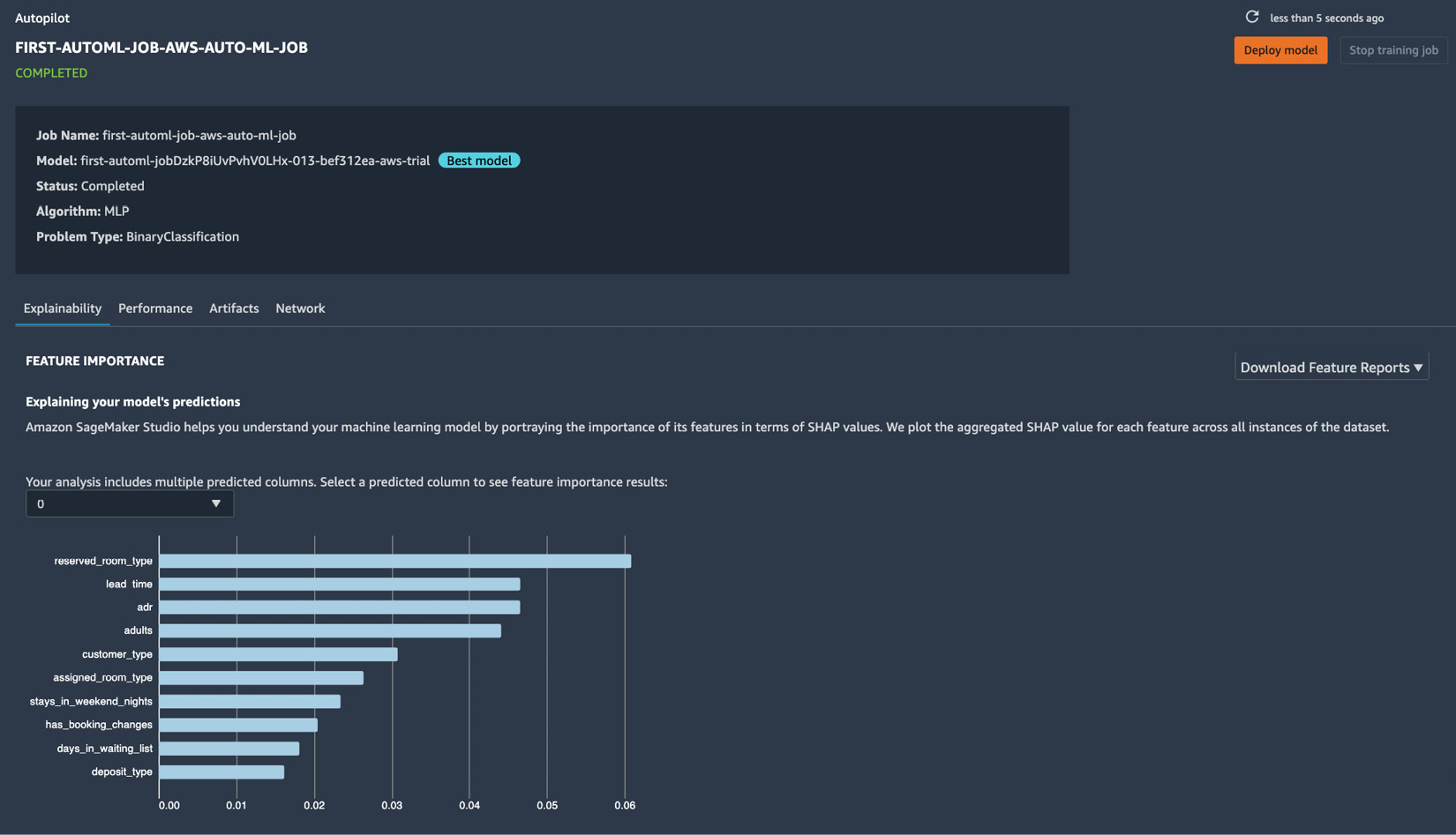
Figure 1.28 – The model details page

Here, we can see that reserved_room_type, lead_time, and adr are the most important features that affect the chance of a hotel booking getting canceled.

Note

Note that you may get a different set of results from what we have in this section.

We should see the following information on the model details page as well:

• Problem type
• Algorithm used
• Location of the input and output artifacts
• Model metric values
• Hyperparameter values used to train the model

Important note

Make sure that you delete the inference endpoint(s) created after running the SageMaker Autopilot experiment. To find the running inference endpoints, simply navigate to https://us-west-2.console.aws.amazon.com/sagemaker/home?region=us-west-2#/endpoints and manually delete the unused resources. Note that the link provided assumes that the inference endpoint has been created in the Oregon (us-west-2) region. We will skip performing sample predictions using the inference endpoint for now. We will cover this, along with deployment strategies, in Chapter 7, SageMaker Deployment Solutions.

At this point, we should have a good grasp of how to use several AutoML solutions such as AutoGluon, SageMaker Canvas, and SageMaker Autopilot. As we saw in the hands-on solutions of this section, we have a significant number of options when using SageMaker Autopilot to influence the process of finding the best model. If we are more comfortable with a simpler UI with fewer options, then we may use SageMaker Canvas instead. If we are more comfortable developing and engineering ML solutions through code, then we can consider using AutoGluon as well.

In this chapter, we got our feet wet by performing multiple AutoML experiments using a variety of services, capabilities, and tools on AWS. This included using AutoGluon within a Cloud9 environment and SageMaker Canvas and SageMaker Autopilot to run AutoML experiments. The solutions presented in this chapter helped us have a better understanding of the fundamental ML and ML engineering concepts as well. We were able to see some of the steps in the ML process in action, such as EDA, train-test split, model training, evaluation, and prediction.

In the next chapter, we will focus on how the AWS Deep Learning AMIs help speed up the ML experimentation process. We will also take a closer look at how AWS pricing works for EC2 instances so that we are better equipped when managing the overall cost of running ML workloads in the cloud.

For more information regarding the topics that were covered in this chapter, check out the following resources:

• AutoGluon: AutoML for Text, Image, and Tabular Data (https://auto.gluon.ai/stable/index.html)
• Automate model development with Amazon SageMaker Autopilot (https://docs.aws.amazon.com/sagemaker/latest/dg/autopilot-automate-model-development.html)
• SageMaker Canvas Pricing (https://aws.amazon.com/sagemaker/canvas/pricing/)
• Machine Learning with Amazon SageMaker Cookbook, by Joshua Arvin Lat (https://www.amazon.com/Machine-Learning-Amazon-SageMaker-Cookbook/dp/1800567030/)