


 Download code from GitHub
Creating the First TikZ Images
This chapter will work with the most basic but essential concepts.
Specifically, our topics are as follows:
- Using the
tikzpictureenvironment - Working with coordinates
- Drawing geometric shapes
- Using colors
This gives us the foundation to move on to more complex drawings in the upcoming chapters.
It’s good if you already know the basics of geometry and coordinates, but we will have a quick look at the parts we need.
By the end of this chapter, you’ll learn how to create colored drawings with lines, rectangles, circles, ellipses, and arcs and how to position them in a coordinate system.
Technical requirements
You need to have LaTeX on your computer, or you can use Overleaf to compile the code examples of this chapter online. Alternatively, you can go with the book’s website, where you can open, edit, and compile all examples. You can find the code for this chapter at https://tikz.org/chapter-02.
The code is also available on GitHub at https://github.com/PacktPublishing/LaTeX-graphics-with-TikZ/tree/main/02-First-steps-creating-TikZ-images.
Using the tikzpicture environment
In the previous chapter, we saw that we basically load TikZ and then use a tikzpicture environment that contains our drawing commands. Let’s go step by step to create a document that will be the base of all our drawings in this chapter. Our goal is to draw a rectangular grid with dotted lines. Such a grid is really beneficial in positioning objects in our pictures later on. I usually start with such a helper grid, make my drawing, and take the grid out in the final version of the drawing.
As it’s one of our first TikZ examples, we will do it step by step and then discuss how it works:
- Open your LaTeX editor. Start with the
standalonedocument class. In the class options, use thetikzoption and define a border of 10 pt:\documentclass[tikz,border=10pt]{standalone} - Begin the document environment:
\begin{document} - Next, begin a
tikzpictureenvironment:\begin{tikzpicture} - Draw a thin, dotted grid from the coordinate (-3,-3) to the coordinate (3,3):
\draw[thin,dotted] (-3,-3) grid (3,3);
- To better see where the horizontal and vertical axis is, let’s draw them with an arrow tip:
\draw[->] (-3,0) -- (3,0);
\draw[->] (0,-3) -- (0,3);
- End the
tikzpictureenvironment:\end{tikzpicture} - End the document:
\end{document}
Compile the document and look at the output:
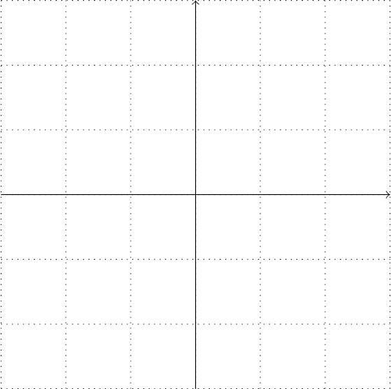
Figure 2.1 – A rectangular grid
In step 1, we used the standalone document class. That class allows us to create documents that consist only of a single drawing and cuts the PDF document to the actual content. Therefore, we don’t have an A4 or letter page with just a tiny drawing, plus a lot of white space and margins.
To get a small margin of 10 pt around the picture, we wrote border=10pt because, with a small margin, it looks nicer in a PDF viewer. Since the standalone class is designed for drawings, it provides a tikz option. As we set that option, the class loads TikZ automatically, so we don’t have to add \usepackage{tikz} anymore.
After we started the document in step 1, we opened a tikzpicture environment in step 3. Every drawing command will happen in this environment until we end it. As it’s a LaTeX environment, it can be used with optional arguments. For example, we could write \begin{tikzpicture}[color=red] to get everything we draw in red unless we specify otherwise. We will talk about valuable options later in this book.
Step 4 was our main task of drawing a grid. We used the \draw command that we will see exceptionally often throughout this book. We specified the following:
- How: We added
thinanddottedoptions in square brackets because that’s the LaTeX syntax for optional arguments. So, everything the\drawcommand does will now be in thin and dotted lines. - Where: We set (-3,-3) as the start coordinate and (3,3) as the end coordinate. We will look thoroughly at the coordinates in the next section.
- What: The
gridelement is like a rectangle where one corner is the start coordinate, to the left of it, and the other corner is the end coordinate, to the right of it. It fills this rectangle with a grid of lines. They are, as we required before, thin and dotted.
\draw produces a path with coordinates and picture elements in between until we end with a semicolon. We can sketch it like the following:
\draw[<style>] <coordinate> <picture element> <coordinate> ... ;
Every path must end with a semicolon. Paths with coordinates, elements, and options can be pretty complex and flexible – the rule to end paths with a semicolon allows TikZ to parse and understand where such paths end and other commands follow.
The lines in a grid have a distance of 1 by default. The optional step argument can change that. For example, you could write grid[step=0.5] or do that right at the beginning as the \draw option, such as the following:
\draw[thin,dotted,step=0.5] <coordinate>
  <picture element> <coordinate> ... ;
In step 5, we have drawn two lines. The picture element here is a straight line between the coordinates given. We use the convenient -- shortcut that stands for a line. The -> style determines that we shall have an arrow tip at the end. In the next section, we will draw many lines.
Finally, we just ended the tikzpicture and document environments.
TikZ, document classes, and figures
In this book, we will focus on TikZ picture creation. Remember that we can use TikZ with any LaTeX class, such as article, book, or report. Furthermore, TikZ pictures can be used in a figure environment with label and caption, just like \includegraphics.
While this section showed a manageable number of commands, we should have a closer look at the concept of coordinates, which is now the topic of our next section.
Working with coordinates
When we want TikZ to place a line, a circle, or any other element on the drawing, we need to tell it where to put it. For this, we use coordinates.
Now, you may remember elementary geometry from school or have looked at a good geometry book. In our case, we will use our knowledge of geometry mainly to position elements in our drawings.
Let’s start with classic geometry and how to use it with TikZ.
Cartesian coordinates
You may remember the Cartesian coordinate system you learned in school. Let’s quickly recap it. In the two dimensions of our drawing, we consider an x axis in the horizontal direction going from left to right and a y axis in the vertical order going from bottom to top. Then, we define a point by its distance to each axis. Let’s look at it in a diagram:
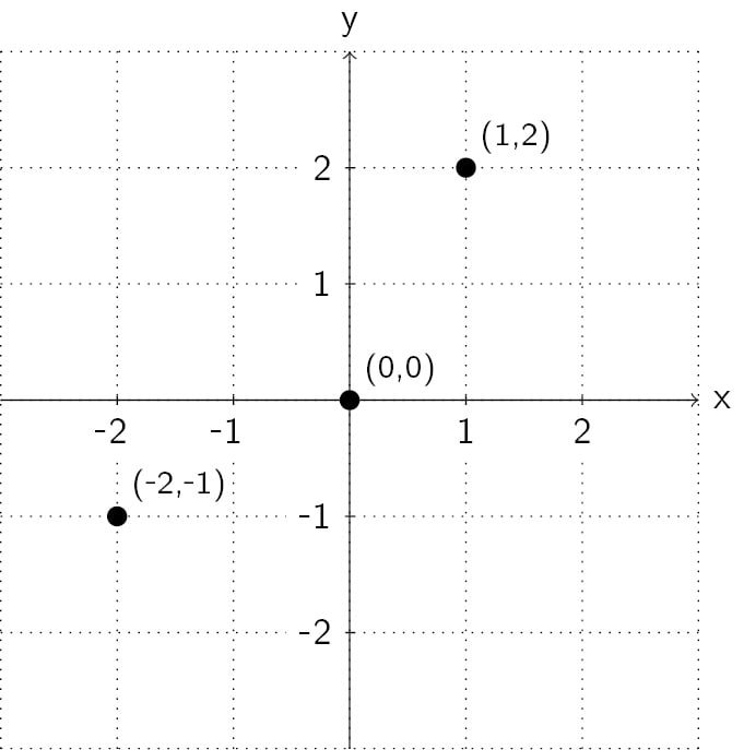
Figure 2.2 – Cartesian coordinate system
In Figure 2.2, we see a point (0,0) that we call the origin. It has a distance of zero to each axis. Then there’s the point, (1,2), that has a distance to the origin in a positive x direction of 1 and a positive y direction of 2. Similarly, for the (-2,1) point, we have an x value of -2, since it goes in the negative direction, and a y value of -1 for the same reason.
Labels at the x axis and y axis and a grid help us to see the dimensions. We will reuse the grid from Figure 2.1 when we next draw lines.
Remember, we draw elements between coordinates, and -- is the code for a line. So, the following command draws a line between the (2,-2) and (2,2) coordinates:
\draw (2,-2) -- (2,2);
We can add more coordinates and lines to this command – let’s make it a square. And to better see it over the grid, let’s make it have very thick blue lines:
\draw[very thick, blue] (-2,-2) -- (-2,2)
  -- (2,2) -- (2,-2) -- cycle;
Here, cycle closes the path, so the last line returns to the first coordinate.
The full context – that is, the complete LaTeX document with the cycle command – is highlighted in the code for Figure 2.1:
\documentclass[tikz,border=10pt]{standalone}
\begin{document}
\begin{tikzpicture}
  \draw[thin,dotted] (-3,-3) grid (3,3);
  \draw[->] (-3,0) -- (3,0);
  \draw[->] (0,-3) -- (0,3);
  \draw[very thick, blue] (-2,-2) -- (-2,2)
    -- (2,2) -- (2,-2) -- cycle;
\end{tikzpicture}
\end{document}
When you compile this document, you get this picture:
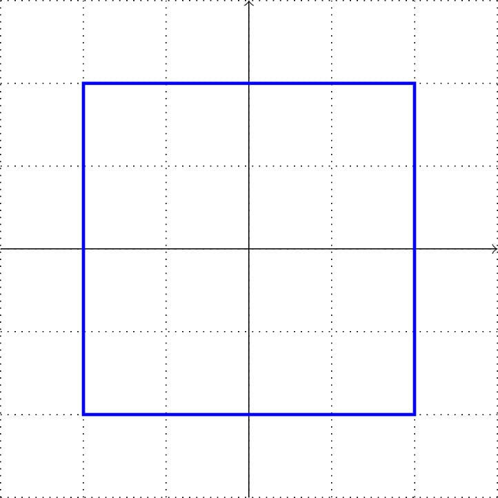
Figure 2.3 – A square in Cartesian coordinates
We used the \draw command to put lines at and between coordinates. How about something else? In TikZ, we can draw a circle with a certain radius as an element, with that radius as an argument in parentheses, such as circle (1) with a radius of 1. Let’s replace the -- lines with that and remove the now unnecessary cycle, and the command now looks like this:
\draw[very thick, blue] (-2,-2) circle (1) (-2,2)
  circle (1) (2,2) circle (1) (2,-2) circle (1);
Compile, and you get this in the PDF document:
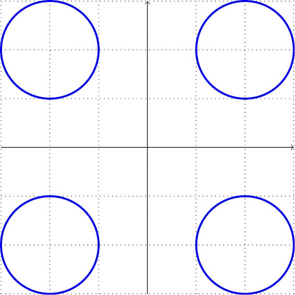
Figure 2.4 – Circles in Cartesian coordinates
This example emphasizes how we use the \draw command – as a sequence of coordinates with picture elements at those coordinates. As you saw, we can draw several elements in a single \draw command.
With Cartesian coordinates, it was easy to draw a square. But how about a pentagon? Or a hexagon? Calculating corner coordinates looks challenging. Here, angle- and distance-based coordinates can be more suitable; let’s look at this next.
Polar coordinates
Let’s consider the same plane as we had in the last section. Just now, we define a point by its distance to the origin and the angle to the x axis. Again, it’s easier to see it in a diagram:
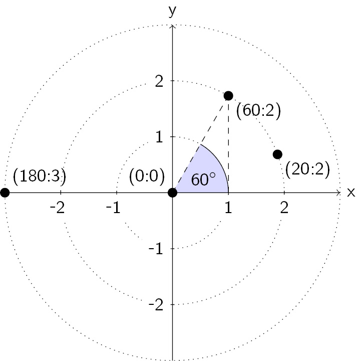
Figure 2.5 – Polar coordinate system
We have a point with the polar coordinates (60:2), which means a distance of 2 from the origin with an angle of 60 degrees to the x axis. TikZ uses a colon to distinguish it from Cartesian coordinates in polar coordinate syntax. The syntax is (angle:distance). So, (20:2) also has a distance of 2 to the origin, (0:0), and an angle of 20 degrees to the x axis, and (180:3) has a distance of 3 and an angle of 180 degrees.
Now, it becomes easier to define points for a hexagon – we specify the angles in multiples of 60 degrees, and all have the same distance from the origin, (0:0); let’s choose 2. Our drawing command becomes as follows:
  \draw[very thick, blue] (0:2) -- (60:2) -- (120:2)
    -- (180:2) --(240:2) -- (300:2) -- cycle;
With the same grid code in the LaTeX document from the previous sections, we get this result from compiling:
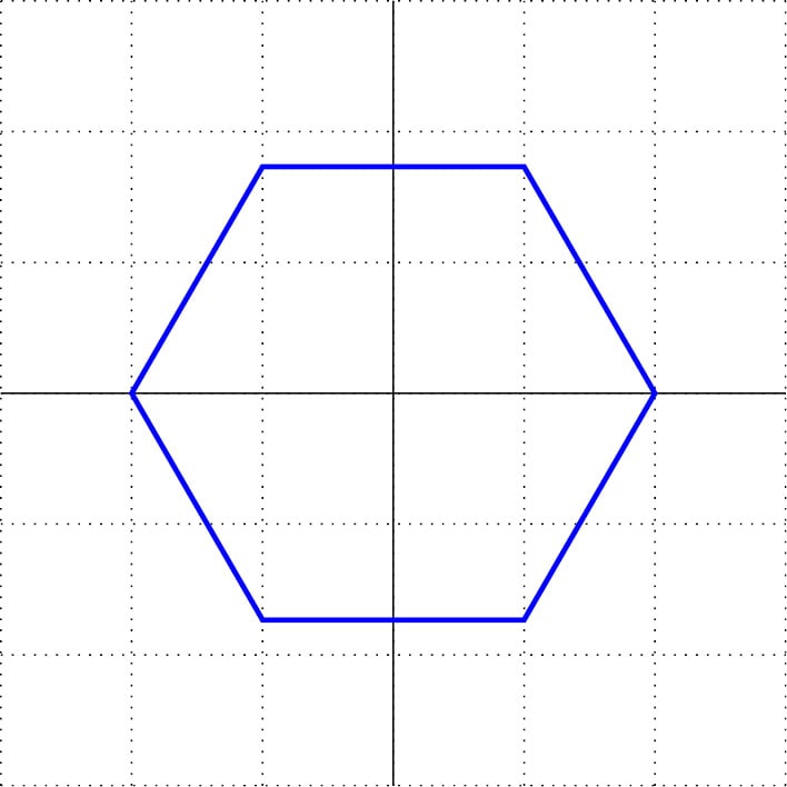
Figure 2.6 – A hexagon in polar coordinates
Polar coordinates are handy when we think of points by distance, rotation, or direction.
Until now, everything was two-dimensional; now, let’s step up by one dimension.
Three-dimensional coordinates
We could use a projection on our drawing plane if we want to draw a cube, a square, or spatial plots. The most famous is isometric projection.
TikZ provides three-dimensional coordinate systems and options. Here is a quick view of how we can use them:
- Specify x, y, and z coordinates that shall be the projection of our three-axis vectors:
\begin{tikzpicture}[x={(0.86cm,0.5cm)},y={(-0.86cm,0.5cm)}, z={(0cm,1cm)}] - Use three coordinates now. We will draw the same square as in Figure 2.3, with
0as the z value, so still in the xy plane:\draw[very thick, blue] (-2,-2,0) -- (-2,2,0)
-- (2,2,0) -- (2,-2,0) -- cycle;
For a better view, we shall again draw axes, as shown in Figure 2.3. Furthermore, we add a circle with a radius of 2. With the necessary aforementioned code highlighted, the full code example is as follows:
\documentclass[tikz,border=10pt]{standalone}
\begin{document}
\sffamily
\begin{tikzpicture}[x={(0.86cm,0.5cm)},
  y={(-0.86cm,0.5cm)}, z={(0cm,1cm)}]
  \draw[very thick, blue] (-2,-2,0) -- (-2,2,0)
   -- (2,2,0) -- (2,-2,0) -- cycle;
  \draw[->] (0,0,0) -- (2.5, 0,  0) node [right] {x};
  \draw[->] (0,0,0) -- (0,  2.5, 0) node [left] {y};
  \draw[->,dashed] (0,0,0) -- (0,  0, 2.5) node [above] {z};
  \draw circle (2);
\end{tikzpicture}
\end{document}
This gives us a skewed view, where the axes and circle help in recognizing it as a 3D isometric view:
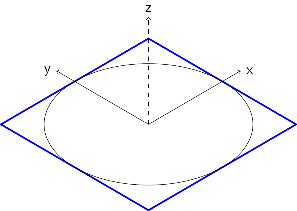
Figure 2.7 – The square and circle in three dimensions
In later chapters, we will work with additional libraries and packages for three-dimensional drawing.
Until now, we have used only absolute coordinates, which refer to the origin and axes. How about a reference to another point, with a distance or angle? We will now look at that.
Using relative coordinates
When we use \draw with a sequence of coordinates, we can state the relative position to the first coordinate by adding a + sign. So, +(4,2) means the new coordinate is plus 4 in the x direction and plus 2 in the y direction. Note that with +, it is always relative to the first coordinate in this path section.
Let’s try this in our code with the grid from Figure 2.3:
\draw[very thick, blue] (-3,-1) -- +(1,0)
  -- +(2,2) -- +(4,2) -- +(5,0) -- +(6,0);
Compile, and you get the following:
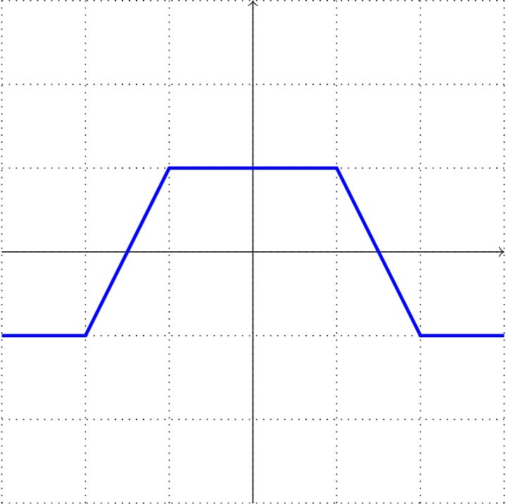
Figure 2.8 – Drawing with relative coordinates
That’s not so handy – always looking back to the first coordinate. Luckily, TikZ offers another syntax with double plus signs. For example, ++(1,2) means plus one in the x direction and plus 2 in the y direction, but from the previous point. That means we can move step by step.
The modified drawing command for the same output is as follows:
\draw[very thick, blue] (-3,-1) -- ++(1,0)
  -- ++(1,2) -- ++(2,0) -- ++(1,-2) -- ++(1,0);
We get the same drawing as shown in Figure 2.8; currently, it’s much easier to follow the movement from one coordinate to the next. That’s why this syntax is pretty popular. Remember that -- here is not the negative version of ++; it’s the line element. The use of -- ++ together can look confusing, but they are two different things – a line and a relative positioning modifier.
Using units
You may already have wondered what a coordinate, (1,2), or a radius of 2 can mean in a document regarding the size of the PDF. Mathematically, in a coordinate system, it’s clear, but in a document, we need actual width, height, and lengths.
So, by default, 1 means 1 cm. You can use any LaTeX dimension, so you can also write (8mm,20pt) as a coordinate or (60:1in) for 60 degrees with a 1-inch distance.
You can change the default unit lengths of 1 cm to any thing else you like. If you write \begin
{tikzpicture}[x=3cm,y=2cm](2,2) would mean the point, (6cm,4cm). It’s an easy way of changing the dimensions of a complete TikZ drawing. For example, change x and y to be twice as big in the tikzpicture options to double a picture in size.
We have now seen how to draw lines, circles, and a grid. Let’s look at more shapes now.
Drawing geometric shapes
We want to progress from high-speed to advanced TikZ concepts, so let’s have a compact summary of what we can draw in this basic setting – that is, we start with \draw <coordinate> (that’s the current coordinate) and continue with some of the following elements:
- Line:
-- (x,y)draws a line from the current coordinate to (x,y). - Rectangle:
rectangle (x,y)draws a rectangle where one corner is the current coordinate, and the opposite corner is (x,y). - Grid: Like
rectanglebut with lines in between as a grid. - Circle:
circle (r)was a short syntax we used previously, but the extended syntax iscircle [radius=r],which draws a circle with the center at the current coordinate and a radius of r. - Ellipse:
ellipse [x radius = rx, y radius = ry]draws an ellipse with a horizontal radius ofrxand a vertical radius ofry. The short form isellipse (rxand ry). - Arc:
arc[start angle=a, end angle=b, radius=r]gives a part of a circle with a radius of r at the current coordinate, starting from angles a to angles b. The short command version isarc(a:b:r).
arc[start angle=a, end angle=b, x radius=rx, y radius=ry] gives a part of an ellipse with an x radius of rx and a y radius of ry at the current coordinate, starting from angle a and going to angle b. The short syntax would be arc(a:b:rx and ry).
Let’s have a few examples to see what these commands do:
- Draw a circle with a radius of
2at the origin:\draw (0,0) circle [radius=2];
- Next, draw an ellipse with a horizontal radius of
0.2and a vertical radius of0.4:\draw (-0.5,0.5,0) ellipse [x radius=0.2, y radius=0.4];
- Now, draw the same ellipse at
(0.5,0.5):\draw (0.5,0.5) ellipse [x radius=0.2, y radius=0.4];
- Next, draw an arc that looks like a smile:
\draw (-1,-1) arc [start angle=185, end angle=355,
x radius=1, y radius=0.5];
- Finally, draw a rectangle with the lower-left corner at
-3,-3and the upper-right corner at3,3:\draw (-3,-3) rectangle (3,3);
When you use all the commands from steps 1 to 5 in a tikzpicture environment and compile, you get the following:
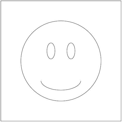
Figure 2.9 – A smiley in a rectangle
This result of the command examples still looks a bit dull. Let’s improve it a bit and fill it with color.
Using colors
We can add colors as options to \draw, as we did for Figure 2.3 when we added blue lines. When we look at circles, ellipses, and rectangles, we can see that the element can have one color while the inner area can have another color. We can add the latter using the fill option.
It’s easier to see it with an example – to draw a blue circle filled with yellow. For this, we can write the following:
\draw[blue,fill=yellow] (0,0) circle [radius=2];
Let’s now fill colors in Figure 2.9. We’ll use fill=yellow for the circle, fill=black for the ellipses, and make the arc thicker by using very thick. Also, let’s omit the rectangle. Our commands are as follows, in a complete document, with the changes highlighted:
\documentclass[tikz,border=10pt]{standalone}
\begin{document}
\begin{tikzpicture}
  \draw[fill=yellow] (0,0) circle [radius=2];
  \draw[fill=black] (-0.5,0.5,0)
    ellipse [x radius=0.2, y radius=0.4];
  \draw[fill=black] (0.5,0.5,0)
    ellipse [x radius=0.2, y radius=0.4];
  \draw[very thick] (-1,-1) arc [start angle=185,
    end angle=355, x radius=1, y radius=0.5];
\end{tikzpicture}
\end{document}
When we compile this document, we get the following:

Figure 2.10 – A smiley with color
TikZ has another way of filling called shading. Instead of filling with a uniform color, shading fills an area with a smooth transition between colors. For our smiley, we chose a predefined ball shading that gives a three-dimensional impression. We set the shading=ball and ball color=yellow options for the face, and ball color=black for the eyes. The code becomes the following:
\draw[shading=ball, ball color=yellow] (0,0)
  circle [radius=2];
\draw[shading=ball, ball color=black] (-0.5,0.5,0)
  ellipse [x radius=0.2, y radius=0.4];
\draw[shading=ball, ball color=black] (0.5,0.5,0)
  ellipse [x radius=0.2, y radius=0.4];
\draw[very thick] (-1,-1) arc [start angle=185,
  end angle=355, x radius=1, y radius=0.5];
Now, our four draw commands produce an even fancier smiley:

Figure 2.11 – A smiley with a three-dimensional appearance
In Chapter 7, Filling, Clipping, and Shading, we will learn more about choosing and mixing colors and explore various ways of filling areas with colors.
Summary
In this chapter, we got used to the basic TikZ syntax, and we learned to draw with different kinds of coordinates. We saw how to draw lines, rectangles, grids, circles, ellipses, and arcs, and how to color them.
Combining text and shapes with alignment options is even more important and worthwhile. That’s the concept of nodes, which we will explore in the next chapter.
Further reading
The TikZ manual includes some excellent tutorials in Part I, Tutorials and Guidelines. You can find the manual at https://texdoc.org/pkg/tikz in PDF format and https://tikz.dev/tutorials-guidelines.
Coordinates and coordinate systems are explained in depth in Part III, Section 13, Specifying Coordinates, and online at https://tikz.dev/tikz-coordinates.
The geometric shapes we learned to draw in this chapter are called path operations in the TikZ manual. Part III, Section 14, Syntax for Path Specifications, is the reference for them. You can read that section online at https://tikz.dev/tikz-paths.

