


In this chapter, we will cover the following topics:
Introducing the IPython notebook
Getting started with exploratory data analysis in IPython
Introducing the multidimensional array in NumPy for fast array computations
Creating an IPython extension with custom magic commands
Mastering IPython's configuration system
Creating a simple kernel for IPython
This book targets intermediate to advanced users who are familiar with Python, IPython, and scientific computing. In this chapter, we will give a brief recap on the fundamental tools we will be using throughout this book: IPython, the notebook, pandas, NumPy, and matplotlib.
In this introduction, we will give a broad overview of IPython and the Python scientific stack for high-performance computing and data science.
IPython is an open source platform for interactive and parallel computing. It offers powerful interactive shells and a browser-based notebook. The notebook combines code, text, mathematical expressions, inline plots, interactive plots, and other rich media within a sharable web document. This platform provides an ideal framework for interactive scientific computing and data analysis. IPython has become essential to researchers, data scientists, and teachers.
IPython can be used with the Python programming language, but the platform also supports many other languages such as R, Julia, Haskell, or Ruby. The architecture of the project is indeed language-agnostic, consisting of messaging protocols and interactive clients (including the browser-based notebook). The clients are connected to kernels that implement the core interactive computing facilities. Therefore, the platform can be useful to technical and scientific communities that use languages other than Python.
In July 2014, Project Jupyter was announced by the IPython developers. This project will focus on the language-independent parts of IPython (including the notebook architecture), whereas the name IPython will be reserved to the Python kernel. In this book, for the sake of simplicity, we will just use the term IPython to refer to either the platform or the Python kernel.
Python is a high-level general-purpose language originally conceived by Guido van Rossum in the late 1980s (the name was inspired by the British comedy Monty Python's Flying Circus). This easy-to-use language is the basis of many scripting programs that glue different software components (glue language) together. In addition, Python comes with an extremely rich standard library (the batteries included philosophy), which covers string processing, Internet Protocols, operating system interfaces, and many other domains.
In the late 1990s, Travis Oliphant and others started to build efficient tools to deal with numerical data in Python: Numeric, Numarray, and finally, NumPy. SciPy, which implements many numerical computing algorithms, was also created on top of NumPy. In the early 2000s, John Hunter created matplotlib to bring scientific graphics to Python. At the same time, Fernando Perez created IPython to improve interactivity and productivity in Python. All the fundamental tools were here to turn Python into a great open source high-performance framework for scientific computing and data analysis.
Note
It is worth noting that Python as a platform for scientific computing was built slowly, step-by-step, on top of a programming language that was not originally designed for this purpose. This fact might explain a few minor inconsistencies or weaknesses of the platform, which do not preclude it from being one of the most popular open frameworks for scientific computing at this time. (You can also refer to http://cyrille.rossant.net/whats-wrong-with-scientific-python/.)
Notable competing open source platforms for numerical computing and data analysis include R (which focuses on statistics) and Julia (a young, high-level language that focuses on high performance and parallel computing). We will see these two languages very briefly in this book, as they can be used from the IPython notebook.
In the late 2000s, Wes McKinney created pandas for the manipulation and analysis of numerical tables and time series. At the same time, the IPython developers started to work on a notebook client inspired by mathematical software such as Sage, Maple, and Mathematica. Finally, IPython 0.12, released in December 2011, introduced the HTML-based notebook that has now gone mainstream.
In 2013, the IPython team received a grant from the Sloan Foundation and a donation from Microsoft to support the development of the notebook. IPython 2.0, released in early 2014, brought many improvements and long-awaited features.
Here is a short summary of the changes brought by IPython 2.0 (succeeding v1.1):
The notebook comes with a new modal user interface:
In the edit mode, we can edit a cell by entering code or text.
In the command mode, we can edit the notebook by moving cells around, duplicating or deleting them, changing their types, and so on. In this mode, the keyboard is mapped to a set of shortcuts that let us perform notebook and cell actions efficiently.
Notebook widgets are JavaScript-based GUI widgets that interact dynamically with Python objects. This major feature considerably expands the possibilities of the IPython notebook. Writing Python code in the notebook is no longer the only possible interaction with the kernel. JavaScript widgets and, more generally, any JavaScript-based interactive element, can now interact with the kernel in real-time.
We can now open notebooks in different subfolders with the dashboard, using the same server. A REST API maps local URIs to the filesystem.
Notebooks are now signed to prevent untrusted code from executing when notebooks are opened.
The dashboard now contains a Running tab with the list of running kernels.
The tooltip now appears when pressing Shift + Tab instead of Tab.
Notebooks can be run in an interactive session via
%run notebook.ipynb.The
%pylabmagic is discouraged in favor of%matplotlib inline(to embed figures in the notebook) andimport matplotlib.pyplot as plt. The main reason is that%pylabclutters the interactive namespace by importing a huge number of variables. Also, it might harm the reproducibility and reusability of notebooks.Python 2.6 and 3.2 are no longer supported. IPython now requires Python 2.7 or >= 3.3.
IPython 3.0 and 4.0, planned for late 2014/early 2015, should facilitate the use of non-Python kernels and provide multiuser capabilities to the notebook.
The Python webpage at www.python.org
Python on Wikipedia at http://en.wikipedia.org/wiki/Python_%28programming_language%29
Python's standard library present at https://docs.python.org/2/library/
Guido van Rossum on Wikipedia at http://en.wikipedia.org/wiki/Guido_van_Rossum
Conversation with Guido van Rossum on the birth of Python available at www.artima.com/intv/pythonP.html
History of scientific Python available at http://fr.slideshare.net/shoheihido/sci-pyhistory
What's new in IPython 2.0 at http://ipython.org/ipython-doc/2/whatsnew/version2.0.html
IPython on Wikipedia at http://en.wikipedia.org/wiki/IPython
History of the IPython notebook at http://blog.fperez.org/2012/01/ipython-notebook-historical.html
The notebook is the flagship feature of IPython. This web-based interactive environment combines code, rich text, images, videos, animations, mathematics, and plots into a single document. This modern tool is an ideal gateway to high-performance numerical computing and data science in Python. This entire book has been written in the notebook, and the code of every recipe is available as a notebook on the book's GitHub repository at https://github.com/ipython-books/cookbook-code.
In this recipe, we give an introduction to IPython and its notebook. In Getting ready, we also give general instructions on installing IPython and the Python scientific stack.
You will need Python, IPython, NumPy, pandas, and matplotlib in this chapter. Together with SciPy and SymPy, these libraries form the core of the Python scientific stack (www.scipy.org/about.html).
Note
You will find full detailed installation instructions on the book's GitHub repository at https://github.com/ipython-books/cookbook-code.
We only give a summary of these instructions here; please refer to the link above for more up-to-date details.
If you're just getting started with scientific computing in Python, the simplest option is to install an all-in-one Python distribution. The most common distributions are:
Anaconda (free or commercial license) available at http://store.continuum.io/cshop/anaconda/
Canopy (free or commercial license) available at www.enthought.com/products/canopy/
Python(x,y), a free distribution only for Windows, available at https://code.google.com/p/pythonxy/
We highly recommend Anaconda. These distributions contain everything you need to get started. You can also install additional packages as needed. You will find all the installation instructions in the links mentioned previously.
Note
Throughout the book, we assume that you have installed Anaconda. We may not be able to offer support to readers who use another distribution.
Alternatively, if you feel brave, you can install Python, IPython, NumPy, pandas, and matplotlib manually. You will find all the instructions on the following websites:
Python is the programming language underlying the ecosystem. The instructions are available at www.python.org/.
IPython provides tools for interactive computing in Python. The instructions for installation are available at http://ipython.org/install.html.
NumPy/SciPy are used for numerical computing in Python. The instructions for installation are available at www.scipy.org/install.html.
pandas provides data structures and tools for data analysis in Python. The instructions for installation are available at http://pandas.pydata.org/getpandas.html.
matplotlib helps in creating scientific figures in Python. The instructions for installation are available at http://matplotlib.org/index.html.
Note
Python 2 or Python 3?
Though Python 3 is the latest version at this date, many people are still using Python 2. Python 3 has brought backward-incompatible changes that have slowed down its adoption. If you are just getting started with Python for scientific computing, you might as well choose Python 3. In this book, all the code has been written for Python 3, but it also works with Python 2. We will give more details about this question in Chapter 2, Best Practices in Interactive Computing.
Once you have installed either an all-in-one Python distribution (again, we highly recommend Anaconda), or Python and the required packages, you can get started! In this book, the IPython notebook is used in almost all recipes. This tool gives you access to Python from your web browser. We covered the essentials of the notebook in the Learning IPython for Interactive Computing and Data Visualization book. You can also find more information on IPython's website (http://ipython.org/ipython-doc/stable/notebook/index.html).
To run the IPython notebook server, type ipython notebook in a terminal (also called the command prompt). Your default web browser should open automatically and load the 127.0.0.1:8888 address. Then, you can create a new notebook in the dashboard or open an existing notebook. By default, the notebook server opens in the current directory (the directory you launched the command from). It lists all the notebooks present in this directory (files with the .ipynb extension).
We assume that a Python distribution is installed with IPython and that we are now in an IPython notebook. We type the following command in a cell, and press Shift + Enter to evaluate it:
In [1]: print("Hello world!")
Hello world!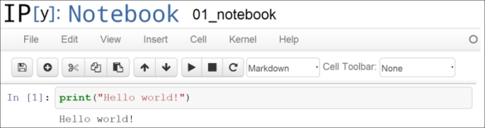
Screenshot of the IPython notebook
A notebook contains a linear succession of cells and output areas. A cell contains Python code, in one or multiple lines. The output of the code is shown in the corresponding output area.
Now, we do a simple arithmetic operation:
In [2]: 2+2
Out[2]: 4
The result of the operation is shown in the output area. Let's be more precise. The output area not only displays the text that is printed by any command in the cell, but it also displays a text representation of the last returned object. Here, the last returned object is the result of
2+2, that is,4.In the next cell, we can recover the value of the last returned object with the
_(underscore) special variable. In practice, it might be more convenient to assign objects to named variables such as inmyresult = 2+2.In [3]: _ * 3 Out[3]: 12
IPython not only accepts Python code, but also shell commands. These commands are defined by the operating system (mainly Windows, Linux, and Mac OS X). We first type
!in a cell before typing the shell command. Here, assuming a Linux or Mac OS X system, we get the list of all the notebooks in the current directory:In [4]: !ls *.ipynb notebook1.ipynb ...
On Windows, you should replace
lswithdir.IPython comes with a library of magic commands. These commands are convenient shortcuts to common actions. They all start with
%(the percent character). We can get the list of all magic commands with%lsmagic:In [5]: %lsmagic Out[5]: Available line magics: %alias %alias_magic %autocall %automagic %autosave %bookmark %cd %clear %cls %colors %config %connect_info %copy %ddir %debug %dhist %dirs %doctest_mode %echo %ed %edit %env %gui %hist %history %install_default_config %install_ext %install_profiles %killbgscripts %ldir %less %load %load_ext %loadpy %logoff %logon %logstart %logstate %logstop %ls %lsmagic %macro %magic %matplotlib %mkdir %more %notebook %page %pastebin %pdb %pdef %pdoc %pfile %pinfo %pinfo2 %popd %pprint %precision %profile %prun %psearch %psource %pushd %pwd %pycat %pylab %qtconsole %quickref %recall %rehashx %reload_ext %ren %rep %rerun %reset %reset_selective %rmdir %run %save %sc %store %sx %system %tb %time %timeit %unalias %unload_ext %who %who_ls %whos %xdel %xmode Available cell magics: %%! %%HTML %%SVG %%bash %%capture %%cmd %%debug %%file %%html %%javascript %%latex %%perl %%powershell %%prun %%pypy %%python %%python3 %%ruby %%script %%sh %%svg %%sx %%system %%time %%timeit %%writefile
Cell magics have a
%%prefix; they concern entire code cells.For example, the
%%writefilecell magic lets us create a text file easily. This magic command accepts a filename as an argument. All the remaining lines in the cell are directly written to this text file. Here, we create a filetest.txtand writeHello world!in it:In [6]: %%writefile test.txt Hello world! Writing test.txt In [7]: # Let's check what this file contains. with open('test.txt', 'r') as f: print(f.read()) Hello world!As we can see in the output of
%lsmagic, there are many magic commands in IPython. We can find more information about any command by adding?after it. For example, to get some help about the%runmagic command, we type%run?as shown here:In [9]: %run? Type: Magic function Namespace: IPython internal ... Docstring: Run the named file inside IPython as a program. [full documentation of the magic command...]
We covered the basics of IPython and the notebook. Let's now turn to the rich display and interactive features of the notebook. Until now, we have only created code cells (containing code). IPython supports other types of cells. In the notebook toolbar, there is a drop-down menu to select the cell's type. The most common cell type after the code cell is the Markdown cell.
Markdown cells contain rich text formatted with Markdown, a popular plain text-formatting syntax. This format supports normal text, headers, bold, italics, hypertext links, images, mathematical equations in LaTeX (a typesetting system adapted to mathematics), code, HTML elements, and other features, as shown here:
### New paragraph This is *rich* **text** with [links](http://ipython.org), equations: $$\hat{f}(\xi) = \int_{-\infty}^{+\infty} f(x)\, \mathrm{e}^{-i \xi x}$$ code with syntax highlighting: ```python print("Hello world!") ``` and images: Running a Markdown cell (by pressing Shift + Enter, for example) displays the output, as shown in the following screenshot:

Rich text formatting with Markdown in the IPython notebook
Note
LaTeX equations are rendered with the
MathJaxlibrary. We can enter inline equations with$...$and displayed equations with$$...$$. We can also use environments such asequation,eqnarray, oralign. These features are very useful to scientific users.By combining code cells and Markdown cells, we can create a standalone interactive document that combines computations (code), text, and graphics.
IPython also comes with a sophisticated display system that lets us insert rich web elements in the notebook. Here, we show how to add HTML, SVG (Scalable Vector Graphics), and even YouTube videos in a notebook.
First, we need to import some classes:
In [11]: from IPython.display import HTML, SVG, YouTubeVideo
We create an HTML table dynamically with Python, and we display it in the notebook:
In [12]: HTML('''
         <table style="border: 2px solid black;">
         ''' +
         ''.join(['<tr>' +
                  ''.join(['<td>{row},{col}</td>'.format(
                                 row=row, col=col
                                 ) for col in range(5)]) +
                  '</tr>' for row in range(5)]) +
         '''
         </table>
         ''')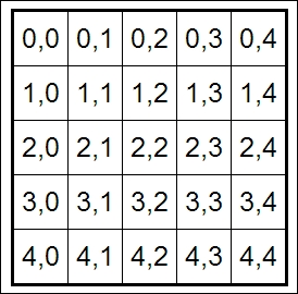
An HTML table in the notebook
Similarly, we can create SVG graphics dynamically:
In [13]: SVG('''<svg width="600" height="80">''' +
         ''.join(['''<circle cx="{x}" cy="{y}" r="{r}"
                             fill="red"
                             stroke-width="2"
                             stroke="black">
                     </circle>'''.format(x=(30+3*i)*(10-i),
                                         y=30,
                                         r=3.*float(i)
                                         ) for i in range(10)]) +
         '''</svg>''')
SVG in the notebook
Finally, we display a YouTube video by giving its identifier to
YoutubeVideo:In [14]: YouTubeVideo('j9YpkSX7NNM')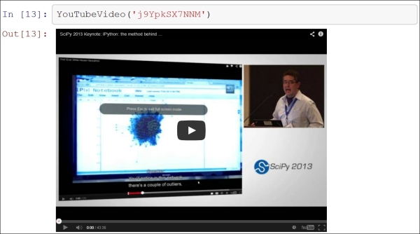
YouTube in the notebook
Now, we illustrate the latest interactive features in IPython 2.0+, namely JavaScript widgets. Here, we create a drop-down menu to select videos:
In [15]: from collections import OrderedDict
         from IPython.display import (display,
                                      clear_output,
                                      YouTubeVideo)
         from IPython.html.widgets import DropdownWidget
In [16]: # We create a DropdownWidget, with a dictionary
         # containing the keys (video name) and the values
         # (Youtube identifier) of every menu item.
         dw = DropdownWidget(values=OrderedDict([
                           ('SciPy 2012', 'iwVvqwLDsJo'),
                           ('PyCon 2012', '2G5YTlheCbw'),
                           ('SciPy 2013', 'j9YpkSX7NNM')]
                                                )
                             )

         # We create a callback function that displays the
         # requested Youtube video.
         def on_value_change(name, val):
             clear_output()
             display(YouTubeVideo(val))

         # Every time the user selects an item, the
         # function `on_value_change` is called, and the
         # `val` argument contains the value of the selected
         # item.
         dw.on_trait_change(on_value_change, 'value')

         # We choose a default value.
         dw.value = dw.values['SciPy 2013']

         # Finally, we display the widget.
         display(dw)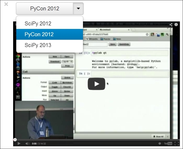
An interactive widget in the notebook
The interactive features of IPython 2.0 bring a whole new dimension to the notebook, and we can expect many developments in the future.
Notebooks are saved as structured text files (JSON format), which makes them easily shareable. Here are the contents of a simple notebook:
{
 "metadata": {
  "name": ""
 },
 "nbformat": 3,
 "nbformat_minor": 0,
 "worksheets": [
  {
   "cells": [
    {
     "cell_type": "code",
     "collapsed": false,
     "input": [
      "print(\"Hello World!\")"
     ],
     "language": "python",
     "metadata": {},
     "outputs": [
      {
       "output_type": "stream",
       "stream": "stdout",
       "text": [
        "Hello World!\n"
       ]
      }
     ],
     "prompt_number": 1
    }
   ],
   "metadata": {}
  }
 ]
}
IPython comes with a special tool, nbconvert, which converts notebooks to other formats such as HTML and PDF (http://ipython.org/ipython-doc/stable/notebook/index.html).
Another online tool, nbviewer, allows us to render a publicly available notebook directly in the browser and is available at http://nbviewer.ipython.org.
We will cover many of these possibilities in the subsequent chapters, notably in Chapter 3, Mastering the Notebook.
Here are a few references about the notebook:
Official page of the notebook available at http://ipython.org/notebook
Documentation of the notebook available at http://ipython.org/ipython-doc/dev/notebook/index.html
Official notebook examples present at https://github.com/ipython/ipython/tree/master/examples/Notebook
User-curated gallery of interesting notebooks available at https://github.com/ipython/ipython/wiki/A-gallery-of-interesting-IPython-Notebooks
Official tutorial on the interactive widgets present at http://nbviewer.ipython.org/github/ipython/ipython/tree/master/examples/Interactive%20Widgets/
In this recipe, we will give an introduction to IPython for data analysis. Most of the subject has been covered in the Learning IPython for Interactive Computing and Data Visualization book, but we will review the basics here.
We will download and analyze a dataset about attendance on Montreal's bicycle tracks. This example is largely inspired by a presentation from Julia Evans (available at http://nbviewer.ipython.org/github/jvns/talks/blob/master/mtlpy35/pistes-cyclables.ipynb). Specifically, we will introduce the following:
Data manipulation with pandas
Data visualization with matplotlib
Interactive widgets with IPython 2.0+
The very first step is to import the scientific packages we will be using in this recipe, namely NumPy, pandas, and matplotlib. We also instruct matplotlib to render the figures as inline images in the notebook:
In [1]: import numpy as np
        import pandas as pd
        import matplotlib.pyplot as plt
        %matplotlib inline
Now, we create a new Python variable called
urlthat contains the address to a CSV (Comma-separated values) data file. This standard text-based file format is used to store tabular data:In [2]: url = "http://donnees.ville.montreal.qc.ca/storage/f/2014-01-20T20%3A48%3A50.296Z/2013.csv"
pandas defines a
read_csv()function that can read any CSV file. Here, we pass the URL to the file. pandas will automatically download and parse the file, and return aDataFrameobject. We need to specify a few options to make sure that the dates are parsed correctly:In [3]: df = pd.read_csv(url, index_col='Date', parse_dates=True, dayfirst=True)The
dfvariable contains aDataFrameobject, a specific pandas data structure that contains 2D tabular data. Thehead(n)method displays the first n rows of this table. In the notebook, pandas displays aDataFrameobject in an HTML table, as shown in the following screenshot:In [4]: df.head(2)
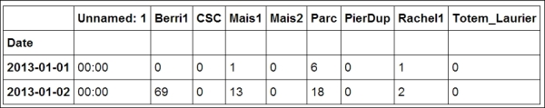
First rows of the DataFrame
Here, every row contains the number of bicycles on every track of the city, for every day of the year.
We can get some summary statistics of the table with the
describe()method:In [5]: df.describe()
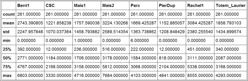
Summary statistics of the DataFrame
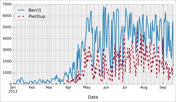
Let's display some figures. We will plot the daily attendance of two tracks. First, we select the two columns,
Berri1andPierDup. Then, we call theplot()method:In [6]: df[['Berri1', 'PierDup']].plot()
Now, we move to a slightly more advanced analysis. We will look at the attendance of all tracks as a function of the weekday. We can get the weekday easily with pandas: the
indexattribute of theDataFrameobject contains the dates of all rows in the table. This index has a few date-related attributes, includingweekday:In [7]: df.index.weekday Out[7]: array([1, 2, 3, 4, 5, 6, 0, 1, 2, ..., 0, 1, 2])
However, we would like to have names (Monday, Tuesday, and so on) instead of numbers between 0 and 6. This can be done easily. First, we create a
daysarray with all the weekday names. Then, we index it bydf.index.weekday. This operation replaces every integer in the index by the corresponding name indays. The first element,Monday, has the index 0, so every 0 indf.index.weekdayis replaced byMondayand so on. We assign this new index to a new column,Weekday, inDataFrame:In [8]: days = np.array(['Monday', 'Tuesday', 'Wednesday', 'Thursday', 'Friday', 'Saturday', 'Sunday']) df['Weekday'] = days[df.index.weekday]To get the attendance as a function of the weekday, we need to group the table elements by the weekday. The
groupby()method lets us do just that. Once grouped, we can sum all the rows in every group:In [9]: df_week = df.groupby('Weekday').sum() In [10]: df_week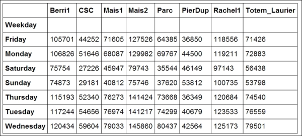
Grouped data with pandas
We can now display this information in a figure. We first need to reorder the table by the weekday using
ix(indexing operation). Then, we plot the table, specifying the line width:In [11]: df_week.ix[days].plot(lw=3) plt.ylim(0); # Set the bottom axis to 0.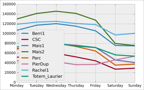
Finally, let's illustrate the new interactive capabilities of the notebook in IPython 2.0. We will plot a smoothed version of the track attendance as a function of time (rolling mean). The idea is to compute the mean value in the neighborhood of any day. The larger the neighborhood, the smoother the curve. We will create an interactive slider in the notebook to vary this parameter in real time in the plot. All we have to do is add the
@interactdecorator above our plotting function:In [12]: from IPython.html.widgets import interact @interact def plot(n=(1, 30)): pd.rolling_mean(df['Berri1'], n).dropna().plot() plt.ylim(0, 8000) plt.show()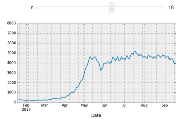
Interactive widget in the notebook
pandas is the right tool to load and manipulate a dataset. Other tools and methods are generally required for more advanced analyses (signal processing, statistics, and mathematical modeling). We will cover these steps in the second part of this book, starting with Chapter 7, Statistical Data Analysis.
Here are some more references about data manipulation with pandas:
Learning IPython for Interactive Computing and Data Visualization, Packt Publishing, our previous book
Python for Data Analysis, O'Reilly Media, by Wes McKinney, the creator of pandas
The documentation of pandas available at http://pandas.pydata.org/pandas-docs/stable/
NumPy is the main foundation of the scientific Python ecosystem. This library offers a specific data structure for high-performance numerical computing: the multidimensional array. The rationale behind NumPy is the following: Python being a high-level dynamic language, it is easier to use but slower than a low-level language such as C. NumPy implements the multidimensional array structure in C and provides a convenient Python interface, thus bringing together high performance and ease of use. NumPy is used by many Python libraries. For example, pandas is built on top of NumPy.
In this recipe, we will illustrate the basic concepts of the multidimensional array. A more comprehensive coverage of the topic can be found in the Learning IPython for Interactive Computing and Data Visualization book.
Let's import the built-in
randomPython module and NumPy:In [1]: import random import numpy as npWe use the
%precisionmagic (defined in IPython) to show only three decimals in the Python output. This is just to reduce the number of digits in the output's text.In [2]: %precision 3 Out[2]: u'%.3f'
We generate two Python lists,
xandy, each one containing 1 million random numbers between 0 and 1:In [3]: n = 1000000 x = [random.random() for _ in range(n)] y = [random.random() for _ in range(n)] In [4]: x[:3], y[:3] Out[4]: ([0.996, 0.846, 0.202], [0.352, 0.435, 0.531])Let's compute the element-wise sum of all these numbers: the first element of
xplus the first element ofy, and so on. We use aforloop in a list comprehension:In [5]: z = [x[i] + y[i] for i in range(n)] z[:3] Out[5]: [1.349, 1.282, 0.733]How long does this computation take? IPython defines a handy
%timeitmagic command to quickly evaluate the time taken by a single statement:In [6]: %timeit [x[i] + y[i] for i in range(n)] 1 loops, best of 3: 273 ms per loop
Now, we will perform the same operation with NumPy. NumPy works on multidimensional arrays, so we need to convert our lists to arrays. The
np.array()function does just that:In [7]: xa = np.array(x) ya = np.array(y) In [8]: xa[:3] Out[8]: array([ 0.996, 0.846, 0.202])The
xaandyaarrays contain the exact same numbers that our original lists,xandy, contained. Those lists were instances of thelistbuilt-in class, while our arrays are instances of thendarrayNumPy class. These types are implemented very differently in Python and NumPy. In this example, we will see that using arrays instead of lists leads to drastic performance improvements.Now, to compute the element-wise sum of these arrays, we don't need to do a
forloop anymore. In NumPy, adding two arrays means adding the elements of the arrays component-by-component. This is the standard mathematical notation in linear algebra (operations on vectors and matrices):In [9]: za = xa + ya za[:3] Out[9]: array([ 1.349, 1.282, 0.733])We see that the
zlist and thezaarray contain the same elements (the sum of the numbers inxandy).Let's compare the performance of this NumPy operation with the native Python loop:
In [10]: %timeit xa + ya
100 loops, best of 3: 10.7 ms per loop
We observe that this operation is more than one order of magnitude faster in NumPy than in pure Python!
Now, we will compute something else: the sum of all elements in
xorxa. Although this is not an element-wise operation, NumPy is still highly efficient here. The pure Python version uses the built-insum()function on an iterable. The NumPy version uses thenp.sum()function on a NumPy array:In [11]: %timeit sum(x) # pure Python %timeit np.sum(xa) # NumPy 100 loops, best of 3: 17.1 ms per loop 1000 loops, best of 3: 2.01 ms per loopWe also observe an impressive speedup here also.
Finally, let's perform one last operation: computing the arithmetic distance between any pair of numbers in our two lists (we only consider the first 1000 elements to keep computing times reasonable). First, we implement this in pure Python with two nested
forloops:In [12]: d = [abs(x[i] - y[j]) for i in range(1000) for j in range(1000)] In [13]: d[:3] Out[13]: [0.230, 0.037, 0.549]Now, we use a NumPy implementation, bringing out two slightly more advanced notions. First, we consider a two-dimensional array (or matrix). This is how we deal with the two indices, i and j. Second, we use broadcasting to perform an operation between a 2D array and 1D array. We will give more details in the How it works... section.
In [14]: da = np.abs(xa[:1000,None] - ya[:1000])
In [15]: da
Out[15]: array([[ 0.23 ,  0.037,  ...,  0.542,  0.323,  0.473],
                 ...,
                [ 0.511,  0.319,  ...,  0.261,  0.042,  0.192]])
In [16]: %timeit [abs(x[i] - y[j])
                  for i in range(1000) for j in range(1000)]
         %timeit np.abs(xa[:1000,None] - ya[:1000])
1 loops, best of 3: 292 ms per loop
100 loops, best of 3: 18.4 ms per loop
Here again, we observe significant speedups.
A NumPy array is a homogeneous block of data organized in a multidimensional finite grid. All elements of the array share the same data type, also called dtype (integer, floating-point number, and so on). The shape of the array is an n-tuple that gives the size of each axis.
A 1D array is a vector; its shape is just the number of components.
A 2D array is a matrix; its shape is (number of rows, number of columns).
The following figure illustrates the structure of a 3D (3, 4, 2) array that contains 24 elements:
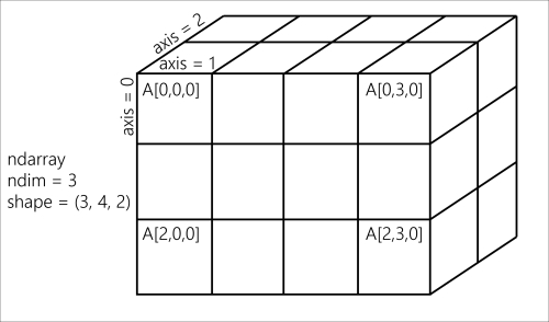
A NumPy array
The slicing syntax in Python nicely translates to array indexing in NumPy. Also, we can add an extra dimension to an existing array, using None or np.newaxis in the index. We used this trick in our previous example.
Element-wise arithmetic operations can be performed on NumPy arrays that have the same shape. However, broadcasting relaxes this condition by allowing operations on arrays with different shapes in certain conditions. Notably, when one array has fewer dimensions than the other, it can be virtually stretched to match the other array's dimension. This is how we computed the pairwise distance between any pair of elements in xa and ya.
How can array operations be so much faster than Python loops? There are several reasons, and we will review them in detail in Chapter 4, Profiling and Optimization. We can already say here that:
In NumPy, array operations are implemented internally with C loops rather than Python loops. Python is typically slower than C because of its interpreted and dynamically-typed nature.
The data in a NumPy array is stored in a contiguous block of memory in RAM. This property leads to more efficient use of CPU cycles and cache.
There's obviously much more to say about this subject. Our previous book, Learning IPython for Interactive Computing and Data Visualization, contains more details about basic array operations. We will use the array data structure routinely throughout this book. Notably, Chapter 4, Profiling and Optimization, covers advanced techniques of using NumPy arrays.
Here are some more references:
Introduction to the
ndarrayon NumPy's documentation available at http://docs.scipy.org/doc/numpy/reference/arrays.ndarray.htmlTutorial on the NumPy array available at http://wiki.scipy.org/Tentative_NumPy_Tutorial
The NumPy array in the SciPy lectures notes present at http://scipy-lectures.github.io/intro/numpy/array_object.html
The Getting started with exploratory data analysis in IPython recipe
The Understanding the internals of NumPy to avoid unnecessary array copying recipe in Chapter 4, Profiling and Optimization
Although IPython comes with a wide variety of magic commands, there are cases where we need to implement custom functionality in a new magic command. In this recipe, we will show how to create line and magic cells, and how to integrate them in an IPython extension.
Let's import a few functions from the IPython magic system:
In [1]: from IPython.core.magic import (register_line_magic,
                                        register_cell_magic)
Defining a new line magic is particularly simple. First, we create a function that accepts the contents of the line (except the initial
%-prefixed name). The name of this function is the name of the magic. Then, we decorate this function with@register_line_magic:In [2]: @register_line_magic def hello(line): if line == 'french': print("Salut tout le monde!") else: print("Hello world!") In [3]: %hello Hello world! In [4]: %hello french Salut tout le monde!Let's create a slightly more useful
%%csvcell magic that parses a CSV string and returns a pandasDataFrameobject. This time, the arguments of the function are the characters that follow%%csvin the first line and the contents of the cell (from the cell's second line to the last).In [5]: import pandas as pd #from StringIO import StringIO # Python 2 from io import StringIO # Python 3 @register_cell_magic def csv(line, cell): # We create a string buffer containing the # contents of the cell. sio = StringIO(cell) # We use pandas' read_csv function to parse # the CSV string. return pd.read_csv(sio) In [6]: %%csv col1,col2,col3 0,1,2 3,4,5 7,8,9 Out[6]: col1 col2 col3 0 0 1 2 1 3 4 5 2 7 8 9We can access the returned object with
_.In [7]: df = _ df.describe() Out[7]: col1 col2 col3 count 3.000000 3.000000 3.000000 mean 3.333333 4.333333 5.333333 ... min 0.000000 1.000000 2.000000 max 7.000000 8.000000 9.000000The method we described is useful in an interactive session. If we want to use the same magic in multiple notebooks or if we want to distribute it, then we need to create an IPython extension that implements our custom magic command. The first step is to create a Python script (
csvmagic.pyhere) that implements the magic. We also need to define a special functionload_ipython_extension(ipython):In [8]: %%writefile csvmagic.py import pandas as pd #from StringIO import StringIO # Python 2 from io import StringIO # Python 3 def csv(line, cell): sio = StringIO(cell) return pd.read_csv(sio) def load_ipython_extension(ipython): """This function is called when the extension is loaded. It accepts an IPython InteractiveShell instance. We can register the magic with the `register_magic_function` method.""" ipython.register_magic_function(csv, 'cell') Overwriting csvmagic.pyOnce the extension module is created, we need to import it into the IPython session. We can do this with the
%load_extmagic command. Here, loading our extension immediately registers our%%csvmagic function in the interactive shell:In [9]: %load_ext csvmagic In [10]: %%csv col1,col2,col3 0,1,2 3,4,5 7,8,9 Out[10]: col1 col2 col3 0 0 1 2 1 3 4 5 2 7 8 9
An IPython extension is a Python module that implements the top-level load_ipython_extension(ipython) function. When the %load_ext magic command is called, the module is loaded and the load_ipython_extension(ipython) function is called. This function is passed the current InteractiveShell instance as an argument. This object implements several methods we can use to interact with the current IPython session.
An interactive IPython session is represented by a (singleton) instance of the InteractiveShell class. This object handles the history, interactive namespace, and most features available in the session.
Within an interactive shell, we can get the current InteractiveShell instance with the get_ipython() function.
The list of all methods of InteractiveShell can be found in the reference API (see link at the end of this recipe). The following are the most important attributes and methods:
The Python extension module needs to be importable when using %load_ext. Here, our module is in the current directory. In other situations, it has to be in the Python path. It can also be stored in ~\.ipython\extensions, which is automatically put in the Python path.
To ensure that our magic is automatically defined in our IPython profile, we can instruct IPython to load our extension automatically when a new interactive shell is launched. To do this, we have to open the ~/.ipython/profile_default/ipython_config.py file and put 'csvmagic' in the c.InteractiveShellApp.extensions list. The csvmagic module needs to be importable. It is common to create a Python package that implements an IPython extension, which itself defines custom magic commands.
Many third-party extensions and magic commands exist, notably cythonmagic, octavemagic, and rmagic, which all allow us to insert non-Python code in a cell. For example, with cythonmagic, we can create a Cython function in a cell and import it in the rest of the notebook.
Here are a few references:
Documentation of IPython's extension system available at http://ipython.org/ipython-doc/dev/config/extensions/
Defining new magic commands explained at http://ipython.org/ipython-doc/dev/interactive/reference.html#defining-magics
Index of IPython extensions at https://github.com/ipython/ipython/wiki/Extensions-Index
API reference of
InteractiveShellavailable at http://ipython.org/ipython-doc/dev/api/generated/IPython.core.interactiveshell.html
IPython implements a truly powerful configuration system. This system is used throughout the project, but it can also be used by IPython extensions. It could even be used in entirely new applications.
In this recipe, we show how to use this system to write a configurable IPython extension. We will create a simple magic command that displays random numbers. This magic command comes with configurable parameters that can be set by the user in their IPython configuration file.
We create an IPython extension in a
random_magics.pyfile. Let's start by importing a few objects.Note
Be sure to put the code in steps 1-5 in an external text file named
random_magics.py, rather than in the notebook's input!from IPython.utils.traitlets import Int, Float, Unicode, Bool from IPython.core.magic import (Magics, magics_class, line_magic) import numpy as np
We create a
RandomMagicsclass deriving fromMagics. This class contains a few configurable parameters:@magics_class class RandomMagics(Magics): text = Unicode(u'{n}', config=True) max = Int(1000, config=True) seed = Int(0, config=True)We need to call the parent's constructor. Then, we initialize a random number generator with a seed:
    def __init__(self, shell):
        super(RandomMagics, self).__init__(shell)
        self._rng = np.random.RandomState(self.seed or None)
We create a
%randomline magic that displays a random number:@line_magic def random(self, line): return self.text.format(n=self._rng.randint(self.max))Finally, we register that magic when the extension is loaded:
def load_ipython_extension(ipython):
    ipython.register_magics(RandomMagics)
Let's test our extension in the notebook:
In [1]: %load_ext random_magics
In [2]: %random
Out[2]: '635'
In [3]: %random
Out[3]: '47'
Our magic command has a few configurable parameters. These variables are meant to be configured by the user in the IPython configuration file or in the console when starting IPython. To configure these variables in the terminal, we can type the following command in a system shell:
ipython --RandomMagics.text='Your number is {n}.' --RandomMagics.max=10 --RandomMagics.seed=1In this session, we get the following behavior:
In [1]: %load_ext random_magics
In [2]: %random
Out[2]: u'Your number is 5.'
In [3]: %random
Out[3]: u'Your number is 8.'
To configure the variables in the IPython configuration file, we have to open the
~/.ipython/profile_default/ipython_config.pyfile and add the following line:c.RandomMagics.text = 'random {n}'After launching IPython, we get the following behavior:
In [4]: %random
Out[4]: 'random 652'
IPython's configuration system defines several concepts:
A user profile is a set of parameters, logs, and command history, which are specific to a user. A user can have different profiles when working on different projects. A
xxxprofile is stored in~/.ipython/profile_xxx, where~is the user's home directory.On Linux, the path is generally
/home/yourname/.ipython/profile_xxxOn Windows, the path is generally
C:\Users\YourName\.ipython\profile_xxx
A configuration object, or
Config, is a special Python dictionary that contains key-value pairs. TheConfigclass derives from Python'sdict.The
HasTraitsclass is a class that can have specialtraitattributes. Traits are sophisticated Python attributes that have a specific type and a default value. Additionally, when a trait's value changes, a callback function is automatically and transparently called. This mechanism allows a class to be notified whenever a trait attribute is changed.A
Configurableclass is the base class of all classes that want to benefit from the configuration system. AConfigurableclass can have configurable attributes. These attributes have default values specified directly in the class definition. The main feature ofConfigurableclasses is that the default values of the traits can be overridden by configuration files on a class-by-class basis. Then, instances ofConfigurablescan change these values at leisure.A configuration file is a Python or JSON file that contains the parameters of
Configurableclasses.
The Configurable classes and configuration files support an inheritance model. A Configurable class can derive from another Configurable class and override its parameters. Similarly, a configuration file can be included in another file.
Here is a simple example of a Configurable class:
from IPython.config.configurable import Configurable
from IPython.utils.traitlets import Float

class MyConfigurable(Configurable):
    myvariable = Float(100.0, config=True)
By default, an instance of the MyConfigurable class will have its myvariable attribute equal to 100. Now, let's assume that our IPython configuration file contains the following lines:
c = get_config()
c.MyConfigurable.myvariable = 123.
Then, the myvariable attribute will default to 123. Instances are free to change this default value after they are instantiated.
The get_config() function is a special function that is available in any configuration file.
Additionally, Configurable parameters can be specified in the command-line interface, as we saw in this recipe.
This configuration system is used by all IPython applications (notably console, qtconsole, and notebook). These applications have many configurable attributes. You will find the list of these attributes in your profile's configuration files.
The Magics class derives from Configurable and can contain configurable attributes. Moreover, magic commands can be defined by methods decorated by @line_magic or @cell_magic. The advantage of defining class magics instead of function magics (as in the previous recipe) is that we can keep a state between multiple magic calls (because we are using a class instead of a function).
Here are a few references:
Configuring and customizing IPython at http://ipython.org/ipython-doc/dev/config/index.html
Detailed overview of the configuration system at http://ipython.org/ipython-doc/dev/development/config.html
Defining custom magics available at http://ipython.org/ipython-doc/dev/interactive/reference.html#defining-magics
The traitlets module available at http://ipython.org/ipython-doc/dev/api/generated/IPython.utils.traitlets.html
The architecture that has been developed for IPython and that will be the core of Project Jupyter is becoming increasingly language independent. The decoupling between the client and kernel makes it possible to write kernels in any language. The client communicates with the kernel via socket-based messaging protocols. Thus, a kernel can be written in any language that supports sockets.
However, the messaging protocols are complex. Writing a new kernel from scratch is not straightforward. Fortunately, IPython 3.0 brings a lightweight interface for kernel languages that can be wrapped in Python.
This interface can also be used to create an entirely customized experience in the IPython notebook (or another client application such as the console). Normally, Python code has to be written in every code cell; however, we can write a kernel for any domain-specific language. We just have to write a Python function that accepts a code string as input (the contents of the code cell), and sends text or rich data as output. We can also easily implement code completion and code inspection.
We can imagine many interesting interactive applications that go far beyond the original use cases of IPython. These applications might be particularly useful for nonprogrammer end users such as high school students.
In this recipe, we will create a simple graphing calculator. The calculator is transparently backed by NumPy and matplotlib. We just have to write functions as y = f(x) in a code cell to get a graph of these functions.
This recipe has been tested on the development version of IPython 3.0. It should work on the final version of IPython 3.0 with no or minimal changes. We give all references about wrapper kernels and messaging protocols at the end of this recipe.
First, we create a
plotkernel.pyfile. This file will contain the implementation of our custom kernel. Let's import a few modules:Note
Be sure to put the code in steps 1-6 in an external text file named
plotkernel.py, rather than in the notebook's input!from IPython.kernel.zmq.kernelbase import Kernel import numpy as np import matplotlib.pyplot as plt from io import BytesIO import urllib, base64
We write a function that returns a base64-encoded PNG representation of a matplotlib figure:
def _to_png(fig):
    """Return a base64-encoded PNG from a
    matplotlib figure."""
    imgdata = BytesIO()
    fig.savefig(imgdata, format='png')
    imgdata.seek(0)
    return urllib.parse.quote(
        base64.b64encode(imgdata.getvalue()))
Now, we write a function that parses a code string, which has the form
y = f(x), and returns a NumPy function. Here,fis an arbitrary Python expression that can use NumPy functions:_numpy_namespace = {n: getattr(np, n) for n in dir(np)} def _parse_function(code): """Return a NumPy function from a string 'y=f(x)'.""" return lambda x: eval(code.split('=')[1].strip(), _numpy_namespace, {'x': x})For our new wrapper kernel, we create a class that derives from
Kernel. There are a few metadata fields we need to provide:class PlotKernel(Kernel): implementation = 'Plot' implementation_version = '1.0' language = 'python' # will be used for # syntax highlighting language_version = '' banner = "Simple plotting"In this class, we implement a
do_execute()method that takes code as input and sends responses to the client:def do_execute(self, code, silent, store_history=True, user_expressions=None, allow_stdin=False): # We create the plot with matplotlib. fig = plt.figure(figsize=(6,4), dpi=100) x = np.linspace(-5., 5., 200) functions = code.split('\n') for fun in functions: f = _parse_function(fun) y = f(x) plt.plot(x, y) plt.xlim(-5, 5) # We create a PNG out of this plot. png = _to_png(fig) if not silent: # We send the standard output to the client. self.send_response(self.iopub_socket, 'stream', { 'name': 'stdout', 'data': 'Plotting {n} function(s)'. \ format(n=len(functions))}) # We prepare the response with our rich data # (the plot). content = { 'source': 'kernel', # This dictionary may contain different # MIME representations of the output. 'data': { 'image/png': png }, # We can specify the image size # in the metadata field. 'metadata' : { 'image/png' : { 'width': 600, 'height': 400 } } } # We send the display_data message with the # contents. self.send_response(self.iopub_socket, 'display_data', content) # We return the execution results. return {'status': 'ok', 'execution_count': self.execution_count, 'payload': [], 'user_expressions': {}, }Finally, we add the following lines at the end of the file:
if __name__ == '__main__':
    from IPython.kernel.zmq.kernelapp import IPKernelApp
    IPKernelApp.launch_instance(kernel_class=PlotKernel)
Our kernel is ready! The next step is to indicate to IPython that this new kernel is available. To do this, we need to create a kernel spec
kernel.jsonfile and put it in~/.ipython/kernels/plot/. This file contains the following lines:{ "argv": ["python", "-m", "plotkernel", "-f", "{connection_file}"], "display_name": "Plot", "language": "python" }The
plotkernel.pyfile needs to be importable by Python. For example, we could simply put it in the current directory.In IPython 3.0, we can launch a notebook with this kernel from the IPython notebook dashboard. There is a drop-down menu at the top right of the notebook interface that contains the list of available kernels. Select the Plot kernel to use it.
Finally, in a new notebook backed by our custom plot kernel, we can simply write the mathematical equation,
y = f(x). The corresponding graph appears in the output area. Here is an example:
Example of our custom plot wrapper kernel
We will give more details about the architecture of IPython and the notebook in Chapter 3, Mastering the Notebook. We will just give a summary here. Note that these details might change in future versions of IPython.
The kernel and client live in different processes. They communicate via messaging protocols implemented on top of network sockets. Currently, these messages are encoded in JSON, a structured, text-based document format.
Our kernel receives code from the client (the notebook, for example). The do_execute()function is called whenever the user sends a cell's code.
The kernel can send messages back to the client with the self.send_response() method:
The data can contain multiple MIME representations: text, HTML, SVG, images, and others. It is up to the client to handle these data types. In particular, the HTML notebook client knows how to represent all these types in the browser.
The function returns execution results in a dictionary.
In this toy example, we always return an ok status. In production code, it would be a good idea to detect errors (syntax errors in the function definitions, for example) and return an error status instead.
All messaging protocol details can be found at the links given at the end of this recipe.
Wrapper kernels can implement optional methods, notably for code completion and code inspection. For example, to implement code completion, we need to write the following method:
def do_complete(self, code, cursor_pos):
    return {'status': 'ok',
            'cursor_start': ...,
            'cursor_end': ...,
            'matches': [...]}
This method is called whenever the user requests code completion when the cursor is at a given cursor_pos location in the code cell. In the method's response, the cursor_start and cursor_end fields represent the interval that code completion should overwrite in the output. The matches field contains the list of suggestions.
These details might have changed by the time IPython 3.0 is released. You will find all up-to-date information in the following references:
Wrapper kernels, available at http://ipython.org/ipython-doc/dev/development/wrapperkernels.html
Messaging protocols, available at http://ipython.org/ipython-doc/dev/development/messaging.html
KernelBase API reference, available at http://ipython.org/ipython-doc/dev/api/generated/IPython.kernel.zmq.kernelbase.html