Search algorithms have various applications in industrial and research-based AI solutions, related to computer vision, machine learning, and robotics. As we progress through the chapters in this book, we will teach you how to use AI in search applications. Searching is something that we do every day, whether we are searching for a song in our filesystem, searching for a friend or colleague on a social network, or finding the best route to a destination. In this chapter, you will learn about the Depth-First Search (DFS) algorithm and develop a file search application.

In this chapter, we will cover the following topics:

• Installing and setting up libraries
• Introducing file search applications
• Formulation of the search problem
• Building search trees with nodes
• Stacks and DFS
• Recursive DFS

Before we get into the basic concepts of searching, we will take a look at the following libraries that have to be installed and how to install them in Windows:

• Python: You can download and install Python libraries from https://www.python.org/downloads/, depending on your operating system
• Graphviz: This open source graph visualization software can be downloaded from http://graphviz.org/download/

• Pip: The tools for installing Python packages are as follows:
  • Pydot: A Python interface to Graphviz's DOT language
  • Matplotlib: This is a Python 2D plotting library

Execute the steps in the following section to install the preceding libraries.

The steps for setting up Python are as follows:

1. For the applications in this book, we'll be using Python 2.7.6, which we can download from https://www.python.org/downloads/.
2. Once an appropriate installer has been downloaded, double-click on it and go ahead with the default options.
3. Based on your operating system, select the Python installer to download, as shown in the following screenshot:

4. The following screenshot shows the location where Python will be installed; make a note of this location:

Now, Python will be installed.

5. The next step is to add Python's path to the Path environment variable. In the System Properties | Advanced tab, click on the Environment Variables... button.
6. In the Environment Variables… window, go to System variables | Path and add the Python location that you made a note of in step 4 (which is C:\Python27 in our case).

7. Now, to check whether Python works, open the Command Prompt and type in the python -- version command. You will get the following output:

The output shown in the preceding screenshot confirms that Python has been installed successfully.

The following steps describe how to set up Graphviz:

1. We can download the graph visualization software from https://graphviz.gitlab.io/download/.
2. Since we are using Windows, we select the option that says Stable 2.38 Windows install packages, as shown in the following screenshot:

Select the .msi downloadable file, shown as follows:

3. Once the Graphviz executable has downloaded, go ahead and install the file with the default options; again, make a note of the path, as shown in the following screenshot:

4. Now, we will add Graphviz's bin folder to the path variable, as we did when installing Python in the previous section. Then, copy the location where Graphviz is installed and append \bin, as shown in the following screenshot:

5. To validate whether this library has been installed properly, open a new Command Prompt window and type the dot -V command, and you will get the following result:

The output shown in the preceding screenshot confirms that Graphviz has been installed successfully.

The steps for installing pip are as follows:

1. To install pip, you need to download the get-pip.py file from https://bootstrap.pypa.io/get-pip.py, and make a note of the path where the file is located. In my case, the file is located at Documents\ai\softwares.
2. Open the Command Prompt and go to the Documents\ai\softwares folder by using the cd command, as shown in the following screenshot:

3. Use the dir command to take a look at the contents of this folder, where you will see get-pip.py, shown in the following screenshot:

4. Next, we'll run the python get-pip.py command.
5. Now, let's add Python's scripts folder to the Path environment variable.
6. Open another Command Prompt window and test the installation of pip by typing the pip --version command. Upon successful installation, you will get the following output:

7. Once pip has installed, you can install pydot by running the following command:

pip install pydot 

8. Finally, install matplotlib by executing the following command:

pip install matplotlib  

9. We can check whether the libraries have been installed properly by using the import command in Python's interpreter, as shown in the following screenshot:

Now, we're done installing the libraries that we will need in Windows for this book . In the next topic, we will look at how we can go about developing a file search application.

In file managers, file searching is used to find files with specific names. In IDEs, file searching is used to find program files with specific code text.

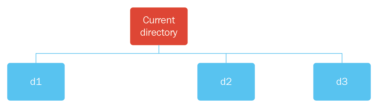
In this topic, we'll develop the first example in order to find a file named f211.txt. The folder structure is shown in the following screenshot:

This folder structure can be represented as a tree, as shown in the following diagram; the file that we're trying to find is shown with a green border:

Let's go ahead and look at how file searching will work to find this file:

1. File searching starts in the current directory; it opens the first folder inside of that (d1) and opens the first folder in d1 (d11). Inside of d11, it compares all of the filenames.
2. Since there's no more content inside of d11, the algorithm gets out of d11, goes inside of d1, and goes for the next folder, which is d12, comparing all of its files.
3. Now, it moves outside of d12 and goes for the next folder inside of d1 (f11), and then the next folder (f12).
4. Now, the search algorithm has covered all of the contents inside of the d1 folder. So, it gets out of d1 and goes for the next folder inside of the current directory, which is d2.
5. Inside of d2, it opens the first folder (d21). Inside of d21, it compares all of the files, and we find the f211 file that we're looking for.

If you refer to the preceding folder structure, you will see that there's a pattern that is being repeated. When we reached f111, the algorithm had explored the leftmost part of the tree, upto its maximum depth. Once the maximum depth was reached, the algorithm backtracked to the previous level and went for the next subtree to the right. Again, in this case, the leftmost part of the subtree is explored, and, when we reach the maximum depth, the algorithm goes for the next subtree. This process is repeated until the file that we are searching for is found.

Now that we understand how the search algorithm functions logically, in the next topic, we will go through the main ingredients of searching, which are used for performing searching in this application.

To understand the functionality of search algorithms, we first need to understand basic searching concepts, such as the state, the ingredients of a search, and the nodes:

• State: The state is defined as the space where the search process takes place. It basically answers the question—what are we searching for? For example, in a navigation application, a state is a place. In our search application, a state is a file or folder.
• Ingredients of a search: There are three main ingredients in a search algorithm. These ingredients are as follows, using the example of a treasure hunt:
  • Initial state: This answers the question—where do we begin our search? In our example, the initial state would be the location where we begin our treasure hunt.
  • Successor function: This answers the question—how do we explore from the initial state? In our example, the successor function should return all of the paths from the location where we began our treasure hunt.
  • Goal function: This answers the question—how will we know when we've found the solution? In our example, the goal function returns true if you've found the place marked as the treasure.

The search ingredients are illustrated in the following diagram:

• Node: A node is the basic unit of a tree. It may consist of data or links to other nodes.

In a file searching application, we start searching from the current directory, so our initial state is the current directory. Now, let's write the code for the state and the initial state, as follows:

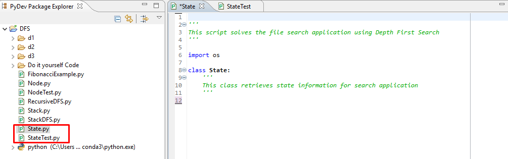
In the preceding screenshot, we have created two Python modules, State.py and StateTest.py. The State.py module will contain the code for the three search ingredients mentioned in the previous section. The StateTest module is a file where we can test these ingredients.

Let's go ahead and create a constructor and a function that returns an initial state, as shown in the following code:

....
import os 

class State:
    '''
    This class retrieves state information for search application
    '''
    
    def __init__(self, path = None):
        if path == None:
            #create initial state
            self.path = self.getInitialState()
        else:
            self.path = path
    
    def getInitialState(self):
        """
        This method returns the current directory
        """
        initialState = os.path.dirname(os.path.realpath(__file__))
        return initialState
 ....

In the preceding code, the following apply:

• We have the constructor (the constructor name) and we have created a property called path, which stores the actual path of the state. In the preceding code example, we can see that the constructor takes path as an argument. The if...else block suggests that if the path is not provided, it will initialize the state as the initial state, and if the path is provided, it will create a state with that particular path.
• The getInitialState() function returns the current working directory.

Now, let's go ahead and create some sample states, as follows:

...
from State import State
import os
import pprint

initialState = State()
print "initialState", initialState.path

interState = State(os.path.join(initialState.path, "d2", "d21"))
goalState = State(os.path.join(initialState.path, "d2", "d21", "f211.txt"))

print "interState", interState.path
print "goalState", goalState.path
....

In the preceding code, we have created the following three states:

• initialState, which points to the current directory
• interState, which is the intermediate function that points to the d21 folder
• goalState, which points to the f211.txt folder

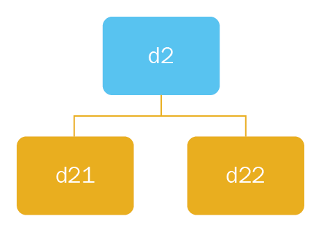
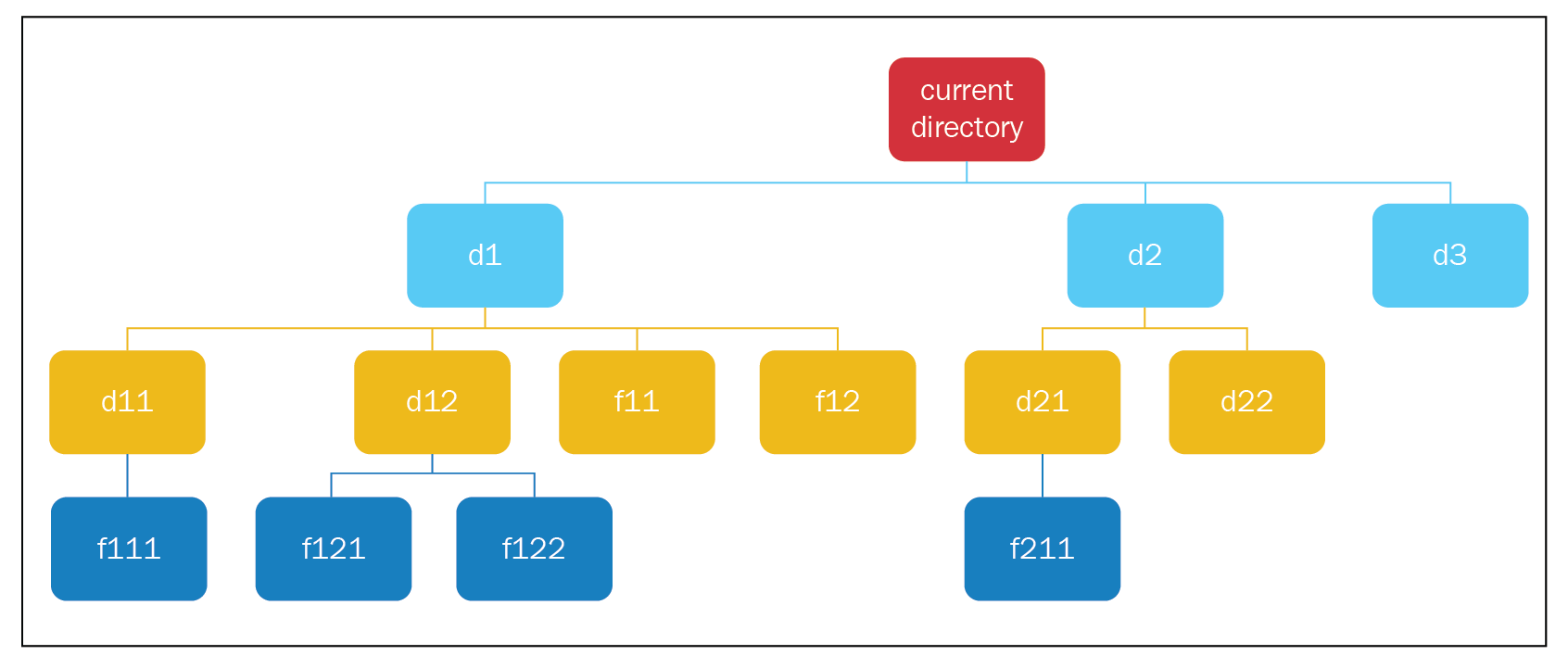
Next, we will look at the successor function. If we're in a particular folder, the successor function should return the folders and files inside of that folder, and, if you're currently looking at a file, it should return an empty array. Considering the following diagram, if the current state is d2, it should return paths to the d21 and d22 folders:

Now, let's create the preceding function with the following code:

...
    def successorFunction(self):
        """
        This is the successor function. It generates all the possible
         paths that can be reached from current path.
        """

        if os.path.isdir(self.path):
            return [os.path.join(self.path, x) for x in         
            sorted(os.listdir(self.path))]
        else:
            return []
...

The preceding function checks whether the current path is a directory. If it is a directory, it gets a sorted list of all of the folders and files inside it, and prepends the current path to them. If it is a file, it returns an empty array.

Now, let's test this function with some input. Open the StateTest module and take a look at the successors to the initial state and intermediate state:

...
initialState = State()
print "initialState", initialState.path

interState = State(os.path.join(initialState.path, "d2", "d21"))
goalState = State(os.path.join(initialState.path, "d2", "d21", "f211.txt"))

print "interState", interState.path
print "goalState", goalState.path
...

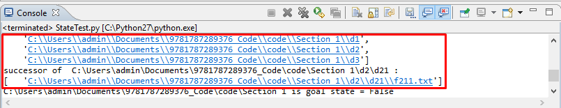
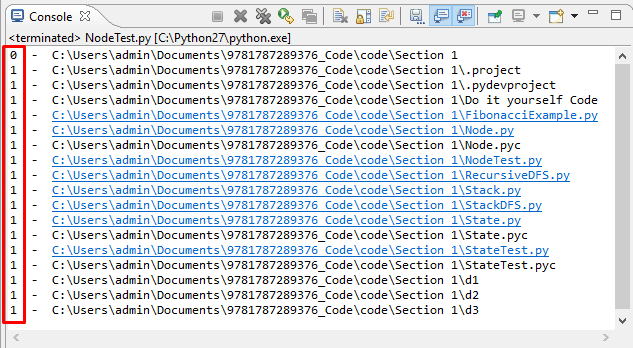
As shown in the preceding code, the successors to the current directory (or the initial state) are the LiClipse project files and the folders d1, d2, and d3, and the successor of the intermediate state is the f211.txt file.

The output of running the preceding code is shown in the following screenshot:

Finally, we will look at the goal function. So, how do we know that we have found the target file, f211.txt? Our goal function should return False for the d21 folder, and True for the f211.txt file . Let's look at how to implement this function in code:

...
def checkGoalState(self):
        """
        This method checks whether the path is goal state 
        """ 
        #check if it is a folder
        if os.path.isdir(self.path):
            return False
        else:
            #extract the filename
            fileSeparatorIndex = self.path.rfind(os.sep)
            filename = self.path[fileSeparatorIndex + 1 : ]
            if filename == "f211.txt":
                return True
            else:
                return False
...

As shown in the preceding code, the function checkGoalState() is our goal function; this checks whether the current path is a directory. Now, since we are looking for a file, this returns False if it's a directory. If it is a file, it extracts the filename from the path. The filename is the substring of the path from the last occurrence of a slash to the end of the string. So, we extract the filename and compare it with f211.txt. If they match, we return True; otherwise, we return False.

Again, let's test this function for the states that we've created. To do so, open the StateTest module, as shown in the following screenshot:

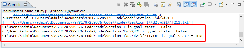
As you can see, the function returns False for the current directory, it returns False for the d21 folder, and it returns True for the f211.txt file.

Now that we understand the three ingredients in search algorithms, in the next section, we will look at building search trees with nodes.

In this topic, you'll be learning how to create a search tree with nodes. We will look at the concepts of states and nodes and the properties and methods of the node class, and we will show you how to create a tree with node objects. In our application, while the state is the path of the file or folder we are processing (for example, the current directory), the node is a node in the search tree (for example, the current directory node).

A node has many properties, and one of them is the state. The other properties are as follows:

• Depth: This is the level of the node in the tree
• Reference to the parent node: This consists of links to the parent node
• References to the child nodes: This consists of links to the child nodes

Let's look at a few examples, in order to understand these concepts more clearly:

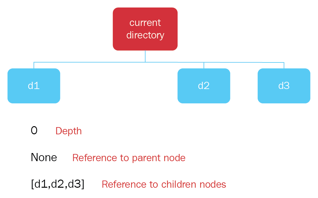
• An example of these concepts in the current directory node is as follows:
  • Depth: 0
  • Reference to parent node: None
  • References to children nodes: d1, d2, d3

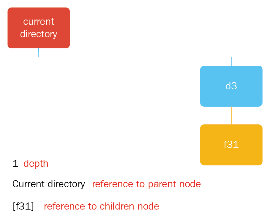
• An example of these concepts in node d3 is as follows:
  • Depth: 1
  • Reference to parent node: Current directory node
  • Reference to children nodes: f31

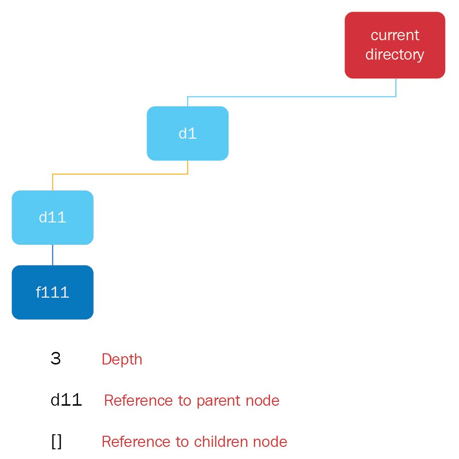
• An example of the concepts for these file node f111 is as follows:
  • Depth: 3
  • Reference to parent node: d11
  • Reference to children node: []

Let's create a class called Node, which includes the four properties that we just discussed:

...
class Node:
    '''
    This class represents a node in the search tree
    '''
    
    def __init__(self, state):
        """
        Constructor
        """
        self.state = state
        self.depth = 0
        self.children = []
        self.parent = None
...

As shown in the preceding code, we have created a class called Node, and this class has a constructor that takes state as an argument. The state argument is assigned to the state property of this node, and the other properties are initialized as follows:

• The depth is set to 0
• The reference to children is set to a blank array
• The reference to parent nodes is set to None

This constructor creates a blank node for the search tree.

Aside from the constructor, we need to create the following two methods:

• addChild(): This method adds a child node under a parent node
• printTree(): This method prints a tree structure

Consider the following code for the addChild() function:

def addChild(self, childNode):
        """
        This method adds a node under another node
        """
        self.children.append(childNode)
        childNode.parent = self
        childNode.depth = self.depth + 1

The addChild() method takes the child node as an argument; the child node is added to the children array, and the parent of the child node is assigned as its parent node. The depth of the child node is the parent node plus one.

Let's look at this in the form of a block diagram for a clearer understanding:

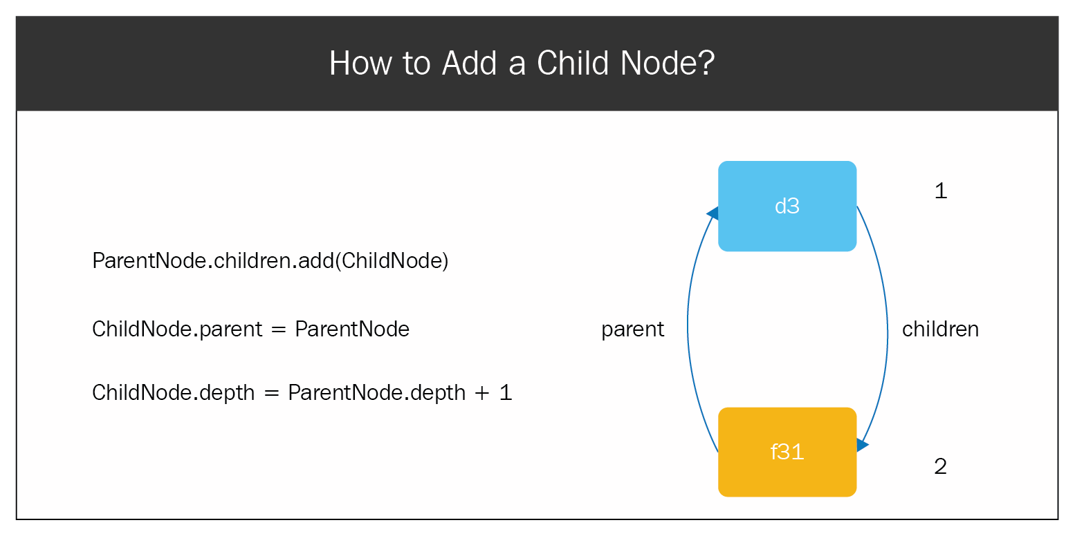
Let's suppose that we're adding node f31 under node d3. So, f31 will be added to the children property of d3, and the parent property of f31 will be assigned as d3. In addition to that, the depth of the child node will be one more than the parent node. Here, the depth of node d3 is 1, so the depth of f31 is 2.

Let's look at the printTree function, as follows:

def printTree(self):
        """
        This method prints the tree
        """
        print self.depth , " - " , self.state.path
        for child in self.children:
            child.printTree()

First, this function prints the depth and the state of the current node; then, it looks through all of its children and calls the printTree method for each of them.

Let's try to create the search tree shown in the following diagram:

As shown in the preceding diagram, as a root node we have the Current directory node; under that node, we have nodes d1, d2, and d3.

We will create a NodeTest module, which will create the sample search tree:

...
from Node import Node
from State import State

initialState = State()
root = Node(initialState)

childStates = initialState.successorFunction()
for childState in childStates:
    childNode = Node(State(childState))
    root.addChild(childNode)
    
root.printTree()
...

As shown in the preceding code, we created an initial state by creating a State object with no arguments, and then we passed this initial state to the Node class constructor, which creates a root node. To get the folders d1, d2, and d3, we called the successorFunction method on the initial state and we looped each of the child states (to create a node from each of them); we added each child node under the root node.

When we execute the preceding code, we get the following output:

Here, we can see that the current directory has a depth of 0, and all of its contents have a depth 1, including d1, d2, and d3.

With that, we have successfully built a sample search tree using the Node class.

In the next topic, you'll be learning about the stack data structure, which will help us to create the DFS algorithm.

A stack is a pile of objects placed one atop another (for example, a stack of books, a stack of clothes, or a stack of papers). There are two stacking operations: one for adding items to a stack, and one for removing items from a stack.

The operation used for adding items to a stack is called push, while the operation used for removing items is called as pop. Items are popped in the reverse order to push; that is why this data structure is called last-in first-out (LIFO).

Let's experiment with the stack data structure in Python. We'll be using the list data structure as a stack in Python. We'll use the append() method to push items to the stack and the pop() method to pop them out:

...
stack = []

print "stack", stack

#add items to the stack
stack.append(1)
stack.append(2)
stack.append(3)
stack.append(4)

print "stack", stack

#pop all the items out
while len(stack) > 0:
    item = stack.pop()
    print item
    
print "stack", stack
...

As shown in the preceding code, we have created an empty stack and we are printing it out. One by one, we are adding the numbers 1, 2, 3, and 4 to the stack and printing them out. Then, one by one, we are popping the items and printing them out; finally, we are printing the remaining stack.

If we execute the preceding code, Stack.py, we get the following output:

Initially, we have an empty stack, and when items 1, 2, 3, and 4 are pushed to the stack, we have 4 at the top of the stack. Now, when you pop the items out, the first one to come out is 4, then 3, then 2, and then 1; this is the reverse of the order of entry. Then, finally, we have an empty stack.

Now that we are clear on how stacks work, let's use these concepts to actually create a DFS algorithm.

Now that you understand the basic concepts of searching, we'll look at how DFS works by using the three basic ingredients of search algorithms—the initial state, the successor function, and the goal function. We will use the stack data structure.

Let's first represent the DFS algorithm in the form of a flowchart, to offer a better understanding:

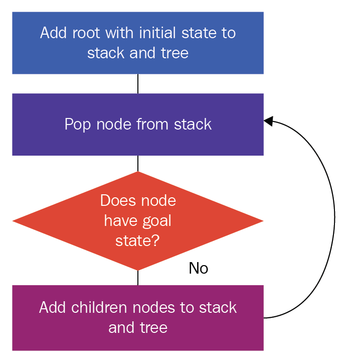
The steps in the preceding flowchart are as follows:

1. We create a root node using the initial state, and we add this to our stack and tree
2. We pop a node from the stack
3. We check whether it has the goal state; if it has the goal state, we stop our search here
4. If the answer to the condition in step 3 is No, then we find the child nodes of the pop node, and add them to the tree and stack
5. We repeat steps 2 to 4 until we either find the goal state or exhaust all of the nodes in the search tree

Let's apply the preceding algorithm to our filesystem, as follows:

1. We create our root node, add it to the search tree, and add it to the stack. We pop a node from the stack, which is the current directory node.
2. The current directory node doesn't have the goal state, so we find its child nodes and add them to the tree and stack.

3. We pop a node from the stack (d1); it doesn't have the goal state, so we find its child nodes and add it to the tree and stack.
4. We pop a node from the stack (d11); it doesn't have the goal state, so we find its child node, add it to the tree and stack.
5. We pop a node (f111); it doesn't have the goal state, and it also doesn't have child nodes, so we carry on.
6. We pop the next node, d12; we find its child nodes and add them to the tree and stack.
7. We pop the next node, f121, and it doesn't have any child nodes, so we carry on.
8. We pop the next node, f122, and it doesn't have any child nodes, so we carry on.
9. We pop the next node, f11, and we encounter the same case (where we have no child nodes), so we carry on; the same goes for f12.
10. We pop the next node, d2, and we find its child nodes and add them to the tree and stack.
11. We pop the next node, d21, and we find its child node and add it to the tree and stack.
12. We pop the next node, f211, and we find that it has the goal state, so we end our search here.

Let's try to implement these steps in code, as follows:

...
from Node import Node
from State import State


def performStackDFS():
    """
    This function performs DFS search using a stack
    """
    #create stack
    stack = []
    
    #create root node and add to stack 
    initialState = State()
    root = Node(initialState)
    stack.append(root)
...

We have created a Python module called StackDFS.py, and it has a method called performStackDFS(). In this method, we have created an empty stack, which will hold all of our nodes, the initialState, a root node containing the initialState, and finally we have added this root node to the stack.

Remember that in Stack.py, we wrote a while loop to process all of the items in the stack. So, in the same way, in this case we will write a while loop to process all of the nodes in the stack:

...
while len(stack) > 0:
        
        #pop top node
        currentNode = stack.pop()
        
        print "-- pop --", currentNode.state.path
        
        #check if this is goal state
        if currentNode.state.checkGoalState():
            print "reached goal state"
            break
            
        #get the child nodes 
        childStates = currentNode.state.successorFunction()
        for childState in childStates:
            childNode = Node(State(childState))
            currentNode.addChild(childNode)

...

As shown in the preceding code, we pop the node from the top of the stack and call it currentNode(), and then we print it so that we can see the order in which the nodes are processed. We check whether the current node has the goal state, and if it does, we end our execution here. If it doesn't have the goal state, we find its child nodes and add it under currentNode, just like we did in NodeTest.py.

We will also add these child nodes to the stack, but in reverse order, using the following for loop:

...
for index in range(len(currentNode.children) - 1, -1, -1):
            stack.append(currentNode.children[index])

#print tree
    print "----------------------"
    root.printTree()
...

Finally, when we exit the while loop, we print the tree. Upon successful execution of the code, we will get the following output:

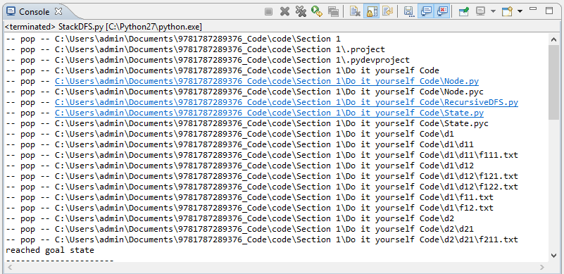
The output displays the order in which the nodes are processed, and we can see the first node of the tree. Finally, we encounter our goal state, and our search stops:

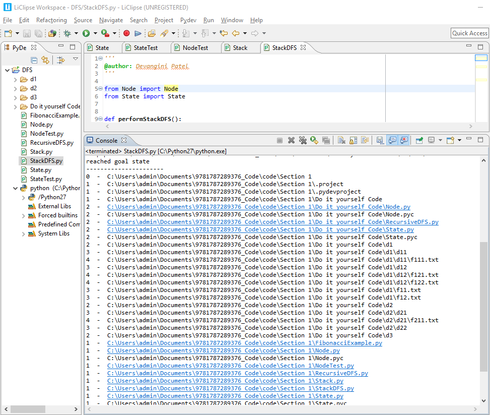
The preceding screenshot displays the search tree. Note that the preceding output and the one before it are almost the same. The only difference is that in the preceding screenshot, we can find two nodes, d22 and d3, because their parent nodes were explored.

When a function calls itself, we say that the function is a recursive function. Let's look at the example of the Fibonacci series. It is defined as follows: f(1) is equal to 1, f(2) is equal to 1, and for n greater than 2, f(n) is equal to f(n-1) + f(n-2). Let's look at the implementation of this function in code, as follows:

...
def fibonacci(n):
    if n <= 2:
        return 1
    else:
        return fibonacci(n-1) + fibonacci(n-2)

print "fibonacci(5)", fibonacci(5)
...

In the preceding code, we have created our function, fibonacci, which takes a number, n, as input. If n is less than or equal to 2, it returns 1; otherwise, it returns fibonacci(n-1) + fibonacci(n-2). Toward the end of the code, we have calculated the value of fibonacci(5), which is 5.

The output of running the preceding code is shown in the following screenshot:

If we want to visualize the recursion tree of the fibonacci function, we can go to https://visualgo.net/en/recursion. This website has visualizations of various data structures and algorithms.

The visualization of a recursion tree is as follows:

As shown in the preceding screenshot, the output that we get here is the same as the output we got with the code, and the order in which the nodes were explored is similar to DFS.

So, what happens when function 1 calls function 2? The program adds a stack frame to the program stack. A stack frame contains the local variables in function 1, the arguments passed to function 1, and the return addresses of function 2 and function 1.

Let's look at the example of the Fibonacci sequence again:

As you can see, the Fibonacci code has been modified for the sake of clarity. Suppose that the program is executing the line in bold, val2 = fibonacci(n-2). Then, the stack frame created will contain the following values—local variables is equal to val1, arguments passed is equal to n, and return address is the address of the code in bold.

This means that the return address points to the unprocessed curve. Because in recursion the program stack keeps a stack of unprocessed calls, instead of storing nodes in the stack, we will call DFS recursively on the child nodes, so that the stack is indirectly maintained.

Let's look at the steps of recursive DFS in the following diagram:

The steps in the preceding diagram are explained as follows:

1. We create an initial state.
2. We create a root node with this initial state.
3. We add the root node to the search tree and call DFS on the root node.
4. Recursive DFS is defined as follows: check whether the node has a goal state. If yes, then it returns the path; if no, then DFS finds the children node, and for each child node DFS adds the node to the tree, finally calling itself on the child node.

Now, we will apply the preceding algorithm to our filesystem, the steps for which are as follows:

1. We create the root node and add it to the search tree, and we call DFS on this root node.
2. When we call DFS on this root node, the function checks whether this node has the goal state, and it doesn't, so it finds its children nodes (d1, d2, and d3). It takes the first node, d1, adds it to the search tree, and calls DFS on the node.
3. When it calls DFS on d1, the function creates a program. When DFS is called on d1, then the program creates a stack frame and adds it to the program stack. In this case, we'll show the remaining nodes to be processed in the for loop. Here, we're adding d2 and d3 in the program stack.

4. When DFS is called on d1, it finds the children nodes d11, d12, f11, and f12, and adds d11 to the search tree.
5. It calls DFS on d11, and when it does so, it creates an entry in the program stack with the unprocessed nodes. Now, when DFS is called on d11, it finds the child node f111, adds f111 to the search tree, and calls DFS on the node.

6. When DFS is called on f111, it has no children nodes, so it returns back; when this happens, the program stack is unwounded, which means that the program returns execution and processes the last unprocessed nodes in the stack. In this case, it starts processing node d12. So, the program adds node d12 to the search tree, and calls DFS on d1.
7. When DFS is called on d12, it finds the children nodes f121 and f122. It adds node f121 to the search tree, and calls DFS on it. When DFS is called on f121, it adds the unprocessed node f122 to the stack.
8. When DFS is called on f121, it has no children nodes, so again the stack is unwounded. So, we process node f122. This node is added to the search tree and DFS is called on it. So, we continue processing the last node, f11, add it to the search tree, and call DFS on it.
9. When we call DFS on f11, it has no children nodes, so again the stack is unwounded. We continue processing node f12, it is added to the search tree, and DFS is called on f12. We encounter this case, and we continue processing node d2. We add it to the search tree, and we call DFS on d2.
10. When we call DFS on d2, we find that is has children nodes: d21 and d22. We add d21 to the search tree, and we call DFS on d21; when we call DFS on d21, it creates an entry for d22. In the program stack, when DFS is called on d21, we find that it has a child, f211. This node is added to the search tree and DFS is called on f211.
11. When DFS is called an f211, we realize that it has the goal state, and we end our search process here.

Let's look at how we can implement recursive DFS, as follows:

...
from State import State
from Node import Node


class RecursiveDFS():
    """
    This performs DFS search
    """
    def __init__(self):
        self.found = False
...

As shown in the preceding code, we have created a Python module called RecursiveDFS.py. It has a class called RecursiveDFS, and, in the constructor, it has a property called found, which indicates whether the solution has been found. We'll look at the significance of the found variable later.

Let's look at the following lines of code:

...
    def search(self):
        """
        This method performs the search
        """
        #get the initial state
        initialState = State()
        
        #create root node
        rootNode = Node(initialState)
        
        #perform search from root node
        self.DFS(rootNode)
        
        rootNode.printTree()
...

Here, we have a method called search, in which we are creating the initialState, and the rootNode we're calling the DFS function on the rootNode. Finally, we print the tree after we perform the DFS search, as follows:

...
def DFS(self, node):
        """
        This creates the search tree
        """
        if not self.found:
            print "-- proc --", node.state.path
            
            #check if we have reached goal state
            if node.state.checkGoalState():
                print "reached goal state"
                #self.found = True
                
            else:
                #find the successor states from current state 
                childStates = node.state.successorFunction()
                
                #add these states as children nodes of current node
                for childState in childStates:
                    childNode = Node(State(childState))
                    node.addChild(childNode)
                    
                    self.DFS(childNode)
....

The DFS function can be defined as follows:

• If the solution has not been found, then the node that is being processed is printed
• We check whether the node has the goal state, and if it does, we print that the goal state has been reached
• If it doesn't have the goal state, we find the child states; next, we create the child node for each child state, we add them to the tree, and we call DFS on each of the child nodes

Let's execute the program; we will get the following output:

When we processed f211, we reached the goal state, but here we have three extra lines; this is because these nodes have been added to the program stack. To remove these lines, we have created a variable called found, so that when the goal state is found, the variable will be set to True. Once we encounter f211, the remaining nodes in the program stack will not be processed:

Let's run this code again and see what happens:

As you can see, once we've processed f211 and reached the goal state, the node processing stops. The output of the printTree function is the same as what we store in StackDFS.py.

Now that you understand how DFS can be made into a recursive function, in the next topic we will look at an application that you can develop by yourself.

In this section, we will look at an application that you can develop by yourself. We will take a look at a new application and discuss the changes that are required. In the Introduction to file search applications section, we discussed two applications of file searching; now, we will develop the second type of example. Our aim is to develop a search application that is able to find program files containing specific program text.

In the code for recursive DFS, we mainly used three classes, as follows:

• State: This has the three main ingredients of the search process
• Node: This is used to build search trees
• Recursive DFS: This has the actual algorithm implementation

Suppose that we want to adapt this code or file search application to new application. We will need to change three methods: getInitialState, successorFunction, and checkGoalState. For the new application of program searching, you will need to change just one method: checkGoalState.

In your new checkGoalState function, you will need to open the file, read the contents of the file line by line, and perform a substring check or regular expression check. Lastly, based on the results of the check, you will return true or false.

So, go ahead and try it out for yourself!

In this chapter, we looked at four basic concepts related to searching: the state, which is the condition of our search process; the node, which is used for building a search tree; the stack, which helps to traverse the search tree and decides the order in which the nodes are traversed; and recursion, which eliminates the need for an explicit stack. You also learned about DFS, which explores the search tree in a depth-first order.

In the next chapter, you'll learn about breadth-first search (BFS), which explores a search tree in a breadth-first order. See you there!