Machine learning (ML) is a subfield of computer science that involves studying and exploring computer algorithms that can learn the structure of data using statistical analysis. The dataset that's used for learning is called training data. The output of training is called a model, which can then be used to run predictions against a new dataset that the model hasn't seen before. There are two broad categories of machine learning: supervised learning and unsupervised learning. In supervised learning, the training dataset is labeled (the dataset will have a target column). The algorithm intends to learn how to predict the target column based on other columns (features) in the dataset. Predicting house prices, stock market changes, and customer churn are some supervised learning examples. In unsupervised learning, on the other hand, the data is not labeled (the dataset will not have a target column). In this, the algorithm intends to recognize the common patterns in the dataset. One of the methods of generating labels for an unlabeled dataset is using unsupervised learning algorithms. Anomaly detection is one of the use cases for unsupervised learning.

The idea of the first mathematical model for machine learning was presented in 1943 by Walter Pitts and Warren McCulloch (The History of Machine Learning: How Did It All Start? – https://labelyourdata.com/articles/history-of-machine-learning-how-did-it-all-start). Later, in the 1950s, Arthur Samuel developed a program for playing championship-level computer checkers. Since then, we have come a long way in ML. I would highly recommend reading this article if you haven't.

Today, as we try to teach real-time decision-making to systems and devices, ML engineer and data scientist positions are the hottest jobs on the market. It is predicted that the global machine learning market will grow from $8.3 billion in 2019 to $117.9 billion by 2027. As shown in the following diagram, it's a unique skill set that overlaps with multiple domains:

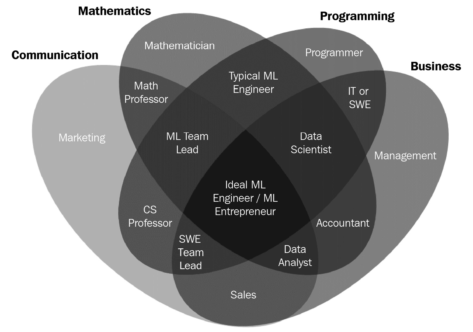
Figure 1.1 – ML/data science skill sets

In 2007 and 2008, the DevOps movement revolutionized the way software was developed and operationalized. It reduced the time to production for software:

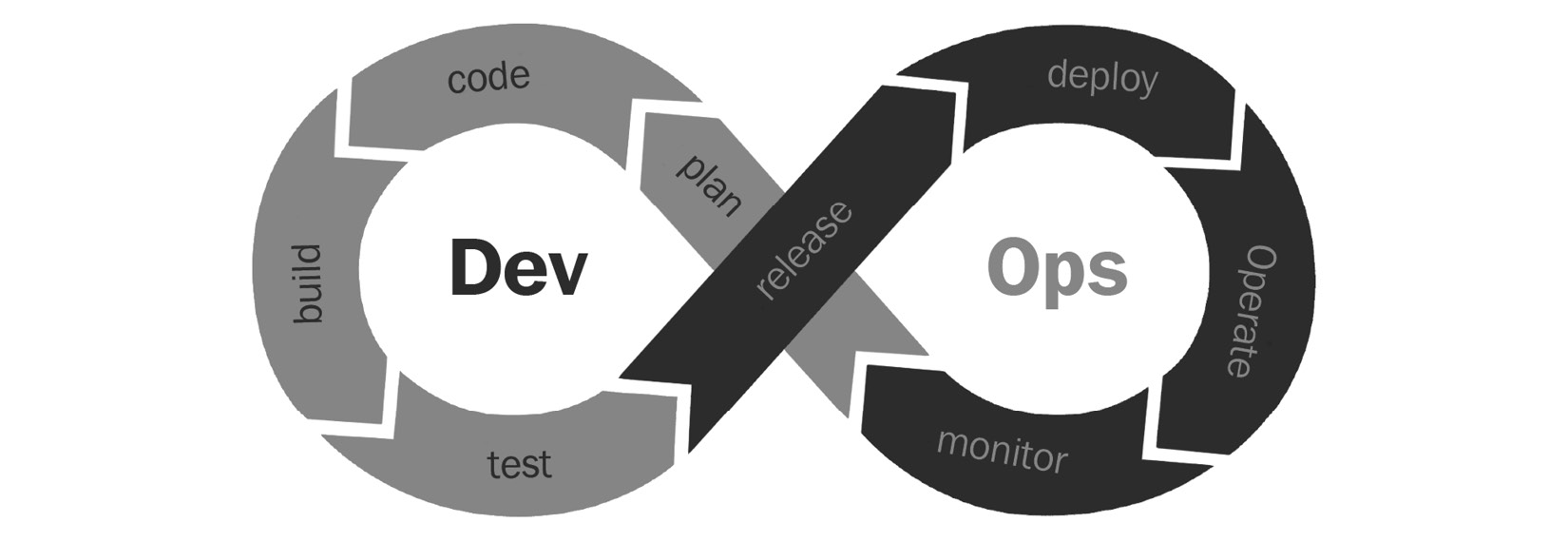
Figure 1.2 – DevOps

Similarly, to take a model from experimentation to operationalization, we need a set of standardized processes that makes this process seamless. Well, the answer to that is machine learning operations (MLOps). Many experts in the industry have come across a set of patterns that would reduce the time to production of ML models. 2021 is the year of MLOps – there are a lot of new start-ups that are trying to cater to the ML needs of the firms that are still behind in the ML journey. We can assume that this will expand over time and only get better, just like any other process. As we grow with it, there will be a lot of discoveries and ways of working, best practices, and more will evolve. In this book, we will talk about one of the common tools that's used to standardize ML and its best practices: the feature store.

Before we discuss what a feature store is and how to use it, we need to understand the ML life cycle and its common oversights. I want to dedicate this chapter to learning about the different stages of the ML life cycle. As part of this chapter, we will take up an ML model-building exercise. We won't dive deep into the ML model itself, such as its algorithms or how to do feature engineering; instead, we will focus on the stages an ML model would typically go through, as well as the difficulties involved in model building versus model operationalization. We will also discuss the stages that are time-consuming and repetitive. The goal of this chapter is to understand the overall ML life cycle and the issues involved in operationalizing models. This will set the stage for later chapters, where we will discuss feature management, the role of a feature store in ML, and how the feature store solves some of the issues we will discuss in this chapter.

In this chapter, we will cover the following topics:

• The ML life cycle in practice
• An ideal world versus the real world
• The most time-consuming stages of ML

Without further ado, let's get our hands dirty with an ML model.

To follow the code examples in this book, you need to be familiar with Python and any notebook environment, which could be a local setup such as Jupyter or an online notebook environment such as Google Colab or Kaggle. We will be using the Python3 interpreter and PIP3 to manage the virtual environment. You can download the code examples for this chapter from the following GitHub link: https://github.com/PacktPublishing/Feature-Store-for-Machine-Learning/tree/main/Chapter01.

As Jeff Daniel's character in HBO's The Newsroom once said, the first step in solving any problem is recognizing there is one. Let's follow this knowledge and see if it works for us.

In this section, we'll pick a problem statement and execute the ML life cycle step by step. Once completed, we'll retrospect and identify any issues. The following diagram shows the different stages of ML:

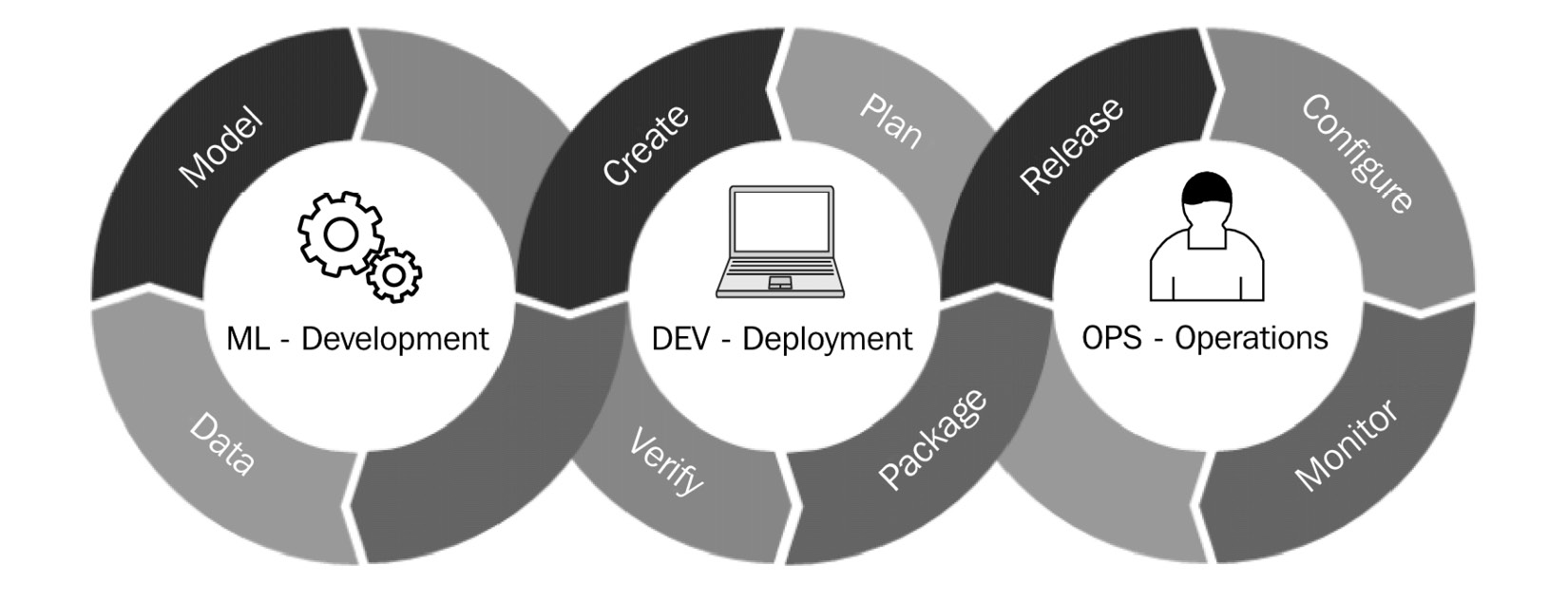
Figure 1.3 – The ML life cycle

Let's take a look at our problem statement.

Problem statement (plan and create)

For this exercise, let's assume that you own a retail business and would like to improve customer experience. First and foremost, you want to find your customer segments and customer lifetime value (LTV). If you have worked in the domain, you probably know different ways to solve this problem. I will follow a medium blog series called Know Your Metrics – Learn what and how to track with Python by Barış Karaman (https://towardsdatascience.com/data-driven-growth-with-python-part-1-know-your-metrics-812781e66a5b). You can go through the article for more details. Feel free to try it out for yourself. The dataset is available here: https://www.kaggle.com/vijayuv/onlineretail.

Data (preparation and cleaning)

First, let's install the pandas package:

!pip install pandas

Let's make the dataset available to our notebook environment. To do that, download the dataset to your local system, then perform either of the following steps, depending on your setup:

• Local Jupyter: Copy the absolute path of the .csv file and give it as input to the pd.read_csv method.
• Google Colab: Upload the dataset by clicking on the folder icon and then the upload icon from the left navigation menu.

Let's preview the dataset:

import pandas as pd

retail_data = pd.read_csv('/content/OnlineRetail.csv', 

                          encoding= 'unicode_escape')

retail_data.sample(5)

The output of the preceding code block is as follows:

Figure 1.4 – Dataset preview

As you can see, the dataset includes customer transaction data. The dataset consists of eight columns, apart from the index column, which is unlabeled:

• InvoiceNo: A unique order ID; the data is of the integer type
• StockCode: The unique ID of the product; the data is of the string type
• Description: The product's description; the data is of the string type
• Quantity: The number of units of the product that have been ordered
• InvoiceDate: The date when the invoice was generated
• UnitPrice: The cost of the product per unit
• CustomerID: The unique ID of the customer who ordered the product
• Country: The country where the product was ordered

Once you have the dataset, before jumping into feature engineering and model building, data scientists usually perform some exploratory analysis. The idea here is to check if the dataset you have is sufficient to solve the problem, identify missing gaps, check if there is any correlation in the dataset, and more.

For the exercise, we'll calculate the monthly revenue and look at its seasonality. The following code block extracts year and month (yyyymm) information from the InvoiceDate column, calculates the revenue property of each transaction by multiplying the UnitPrice and Quantity columns, and aggregates the revenue based on the extracted year-month (yyyymm) column.

Let's continue from the preceding code statement:

##Convert 'InvoiceDate' to of type datetime

retail_data['InvoiceDate'] = pd.to_datetime(

    retail_data['InvoiceDate'], errors = 'coerce')

##Extract year and month information from 'InvoiceDate'

retail_data['yyyymm']=retail_data['InvoiceDate'].dt.strftime('%Y%m')

##Calculate revenue generated per order

retail_data['revenue'] = retail_data['UnitPrice'] * retail_data['Quantity']

## Calculate monthly revenue by aggregating the revenue on year month column  

revenue_df = retail_data.groupby(['yyyymm'])['revenue'].sum().reset_index()

revenue_df.head()

The preceding code will output the following DataFrame:

Figure 1.5 – Revenue DataFrame

Let's visualize the revenue DataFrame. I will be using a library called plotly. The following command will install plotly in your notebook environment:

!pip install plotly

Let's plot a bar graph from the revenue DataFrame with the yyyymm column on the x axis and revenue on the y axis:

import plotly.express as px

##Sort rows on year-month column

revenue_df.sort_values( by=['yyyymm'], inplace=True)

## plot a bar graph with year-month on x-axis and revenue on y-axis, update x-axis is of type category.

fig = px.bar(revenue_df, x="yyyymm", y="revenue", 

             title="Monthly Revenue") 

fig.update_xaxes(type='category')

fig.show()

The preceding codes sort the revenue DataFrame on the yyyymm column and plot a bar graph of revenue against the year-month (yyyymm) column, as shown in the following screenshot. As you can see, September, October, and November are high revenue months. It would have been good to validate our assumption against a few years of data, but unfortunately, we don't have that. Before we move on to model development, let's look at one more metric – the monthly active customers – and see if it's co-related to monthly revenue:

Figure 1.6 – Monthly revenue

Continuing in the same notebook, the following commands will calculate the monthly active customers by aggregating a count of unique CustomerID on the year-month (yyyymm) column:

active_customer_df = retail_data.groupby(['yyyymm'])['CustomerID'].nunique().reset_index()

active_customer_df.columns = ['yyyymm', 

                              'No of Active customers']

active_customer_df.head()

The preceding code will produce the following output:

Figure 1.7 – Monthly active customers DataFrame

Let's plot the preceding DataFrame in the same way that we did for monthly revenue:

## Plot bar graph from revenue data frame with yyyymm column on x-axis and No. of active customers on the y-axis.

fig = px.bar(active_customer_df, x="yyyymm", 

             y="No of Active customers", 

             title="Monthly Active customers") 

fig.update_xaxes(type='category')

fig.show()

The preceding command plots a bar graph of No of Active customers against the year-month (yyyymm) column. As shown in the following screenshot, Monthly Active customers is positively related to the monthly revenue shown in the preceding screenshot:

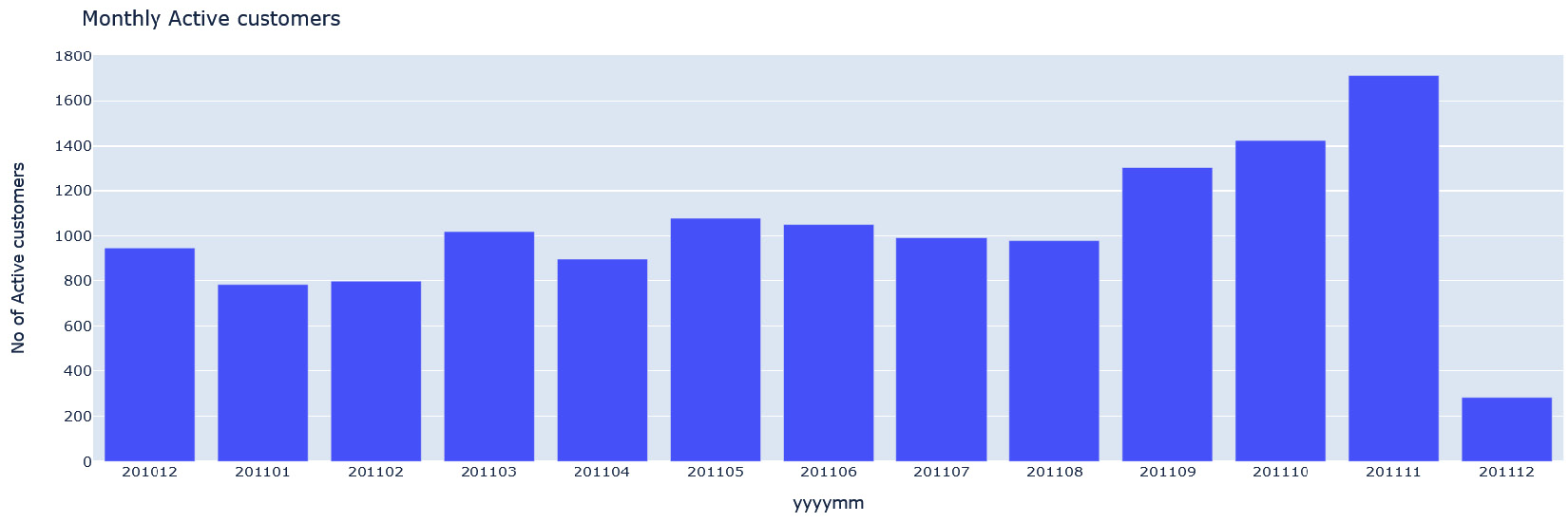
Figure 1.8 – Monthly active customers

In the next section, we'll build a customer LTV model.

Model

Now that we have finished exploring the data, let's build the LTV model. Customer lifetime value (CLTV) is defined as the net profitability associated with a customer's life cycle with the company. Simply put, CLV/LTV is a projection for what each customer is worth to a business (reference: https://www.toolbox.com/marketing/customer-experience/articles/what-is-customer-lifetime-value-clv/). There are different ways to predict lifetime value. One could be predicting the value of a customer, which is a regression problem, while another way could be predicting the customer group, which is a classification problem. In this exercise, we will use the latter approach.

For this exercise, we will segment customers into the following groups:

• Low LTV: Less active or low revenue customers
• Mid-LTV: Fairly active and moderate revenue customers
• High LTV: High revenue customers – the segment that we don't want to lose

We will be using 3 months worth of data to calculate the recency (R), frequency (F), and monetary (M) metrics of the customers to generate features. Once we have these features, we will use 6 months worth of data to calculate the revenue of every customer and generate LTV cluster labels (low LTV, mid-LTV, and high LTV). The generated labels and features will then be used to train an XGBoost model that can be used to predict the group of new customers.

Feature engineering

Let's continue our work in the same notebook, calculate the R, F, and M values for the customers, and group our customers based on a value that's been calculated from the individual R, F, and M scores:

• Recency (R): The recency metric represents how many days have passed since the customer made their last purchase.
• Frequency (F): As the term suggests, F represents how many times the customer made a purchase.
• Monetary (M): How much revenue a particular customer brought in.

Since the spending and purchase patterns of customers differ based on demographic location, we will only consider the data that belongs to the United Kingdom for this exercise. Let's read the OnlineRetails.csv file and filter out the data that doesn't belong to the United Kingdom:

import pandas as pd

from datetime import datetime, timedelta, date

from sklearn.cluster import KMeans

##Read the data and filter out data that belongs to country other than UK

retail_data = pd.read_csv('/content/OnlineRetail.csv', 

                           encoding= 'unicode_escape')

retail_data['InvoiceDate'] = pd.to_datetime(

    retail_data['InvoiceDate'], errors = 'coerce')

uk_data = retail_data.query("Country=='United Kingdom'").reset_index(drop=True)

In the following code block, we will create two different DataFrames. The first one (uk_data_3m) will be for InvoiceDate between 2011-03-01 and 2011-06-01. This DataFrame will be used to generate the RFM features. The second DataFrame (uk_data_6m) will be for InvoiceDate between 2011-06-01 and 2011-12-01. This DataFrame will be used to generate the target column for model training. In this exercise, the target column is LTV groups/clusters. Since we are calculating the customer LTV group, a larger time interval would give a better grouping. Hence, we will be using 6 months worth of data to generate the LTV group labels:

## Create 3months and 6 months data frames

t1 = pd.Timestamp("2011-06-01 00:00:00.054000")

t2 = pd.Timestamp("2011-03-01 00:00:00.054000")

t3 = pd.Timestamp("2011-12-01 00:00:00.054000")

uk_data_3m = uk_data[(uk_data.InvoiceDate < t1) & (uk_data.InvoiceDate >= t2)].reset_index(drop=True)

uk_data_6m = uk_data[(uk_data.InvoiceDate >= t1) & (uk_data.InvoiceDate < t3)].reset_index(drop=True)

Now that we have two different DataFrames, let's calculate the RFM values using the uk_data_3m DataFrame. The following code block calculates the revenue column by multiplying UnitPrice with Quantity. To calculate the RFM values, the code block performs three aggregations on CustomerID:

• To calculate R, max_date in the DataFrame must be calculated and for every customer, we must calculate R = max_date – x.max(), where x.max() calculates the latest InvoiceDate of a specific CustomerID.
• To calculate F, count the number of invoices for a specific CustomerID.
• To calculate M, find the sum value of revenue for a specific CustomerID.

The following code snippet performs this logic:

## Calculate RFM values.

uk_data_3m['revenue'] = uk_data_3m['UnitPrice'] * uk_data_3m['Quantity']

# Calculating the max invoice date in data (Adding additional day to avoid 0 recency value)

max_date = uk_data_3m['InvoiceDate'].max() + timedelta(days=1)

rfm_data = uk_data_3m.groupby(['CustomerID']).agg({

        'InvoiceDate': lambda x: (max_date - x.max()).days,

        'InvoiceNo': 'count',

        'revenue': 'sum'})

rfm_data.rename(columns={'InvoiceDate': 'Recency',

                         'InvoiceNo': 'Frequency',

                         'revenue': 'MonetaryValue'}, 

                         inplace=True)

Here, we have calculated the R, F, and M values for the customers. Next, we need to divide customers into the R, F, and M groups. This grouping defines where a customer stands concerning the other customers in terms of the R, F, and M metrics. To calculate the R, F, and M groups, we will divide the customers into equal-sized groups based on their R, F, and M values, respectively. These were calculated in the previous code block. To achieve this, we will use a method called pd.qcut (https://pandas.pydata.org/pandas-docs/stable/reference/api/pandas.qcut.html) on the DataFrame. Alternatively, you can use any clustering methods to divide customers into different groups. We will add the R, F, and M groups' values together to generate a single value called RFMScore that will range from 0 to 9.

In this exercise, the customers will be divided into four groups. The elbow method (https://towardsdatascience.com/clustering-metrics-better-than-the-elbow-method-6926e1f723a6) can be used to calculate the optimal number of groups for any dataset. The preceding link also contains information about alternative methods you can use to calculate the optimal number of groups, so feel free to try it out. I will leave that as an exercise for you.

The following code block calculates RFMScore:

## Calculate RFM groups of customers 

r_grp = pd.qcut(rfm_data['Recency'], q=4, 

                labels=range(3,-1,-1))

f_grp = pd.qcut(rfm_data['Frequency'], q=4, 

                labels=range(0,4))

m_grp = pd.qcut(rfm_data['MonetaryValue'], q=4, 

                labels=range(0,4))

rfm_data = rfm_data.assign(R=r_grp.values).assign(F=f_grp.values).assign(M=m_grp.values)

rfm_data['R'] = rfm_data['R'].astype(int)

rfm_data['F'] = rfm_data['F'].astype(int)

rfm_data['M'] = rfm_data['M'].astype(int)

rfm_data['RFMScore'] = rfm_data['R'] + rfm_data['F'] + rfm_data['M']

rfm_data.groupby('RFMScore')['Recency','Frequency','MonetaryValue'].mean()

The preceding code will generate the following output:

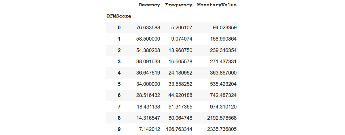
Figure 1.9 – RFM score summary

This summary data gives us a rough idea of how RFMScore is directly proportional to the Recency, Frequency, and MonetaryValue metrics. For example, the group with RFMScore=0 has the highest mean recency (the last purchase day of this group is the farthest in past), the lowest mean frequency, and the lowest mean monetary value. On the other hand, the group with RFMScore=9 has the lowest mean recency, highest mean frequency, and highest mean monetary value.

With that, we understand RFMScore is positively related to the value a customer brings to the business. So, let's segment customers as follows:

• 0-3 => Low value
• 4-6 => Mid value
• 7-9 => High value

The following code labels customers as having either a low, mid, or high value:

# segment customers.

rfm_data['Segment'] = 'Low-Value'

rfm_data.loc[rfm_data['RFMScore']>4,'Segment'] = 'Mid-Value' 

rfm_data.loc[rfm_data['RFMScore']>6,'Segment'] = 'High-Value' 

rfm_data = rfm_data.reset_index()

Customer LTV

Now that we have RFM features ready for the customers in the DataFrame that contains 3 months worth of data, let's use 6 months worth of data (uk_data_6m) to calculate the revenue of the customers, as we did previously, and merge the RFM features with the newly created revenue DataFrame:

# Calculate revenue using the six month dataframe.

uk_data_6m['revenue'] = uk_data_6m['UnitPrice'] * uk_data_6m['Quantity']

revenue_6m = uk_data_6m.groupby(['CustomerID']).agg({

        'revenue': 'sum'})

revenue_6m.rename(columns={'revenue': 'Revenue_6m'}, 

                  inplace=True)

revenue_6m = revenue_6m.reset_index()

revenue_6m = revenue_6m.dropna()

# Merge the 6m revenue data frame with RFM data.

merged_data = pd.merge(rfm_data, revenue_6m, how="left")

merged_data.fillna(0)

Feel free to plot revenue_6m against RFMScore. You will see a positive correlation between the two.

In the flowing code block, we are using the revenue_6m columns, which is the lifetime value of a customer, and creating three groups called Low LTV, Mid LTV, and High LTV using K-means clustering. Again, you can verify the optimal number of clusters using the elbow method mentioned previously:

# Create LTV cluster groups

merged_data = merged_data[merged_data['Revenue_6m']<merged_data['Revenue_6m'].quantile(0.99)]

kmeans = KMeans(n_clusters=3)

kmeans.fit(merged_data[['Revenue_6m']])

merged_data['LTVCluster'] = kmeans.predict(merged_data[['Revenue_6m']])

merged_data.groupby('LTVCluster')['Revenue_6m'].describe()

The preceding code block produces the following output:

Figure 1.10 – LTV cluster summary

As you can see, the cluster with label 1 contains the group of customers whose lifetime value is very high since the mean revenue of the group is $14,123.309, whereas there are only 21 such customers. The cluster with label 0 contains the group of customers whose lifetime value is low since the mean revenue of the group is only $828.67, whereas there are 1,170 such customers. This grouping gives us an idea of which customers should always be kept happy.

The feature set and model

Let's build an XGBoost model using the features we have calculated so far so that the model can predict the LTV group of the customers, given the input features. The following is the final feature set that will be used as input for the model:

feature_data = pd.get_dummies(merged_data)

feature_data.head(5)

The preceding code block produces the following DataFrame. This includes the feature set that will be used to train the model:

Figure 1.11 – Feature set for model training

Now, let's use this feature set to train the Xgboost model. The prediction label (y) is the LTVCluster column; the rest of the dataset except for the Revenue_6m and CustomerID columns are the X value. Revenue_6m will be dropped from the feature set as the LTVCluster column (y) is calculated using Revenue_6m. For the new customer, we can calculate other features without needing at least 6 months worth of data and also predict their LTVCluster(y).

The following code will train the Xgboost model:

from sklearn.metrics import classification_report, confusion_matrix

import xgboost as xgb

from sklearn.model_selection import KFold, cross_val_score, train_test_split

#Splitting data into train and test data set.

X = feature_data.drop(['CustomerID', 'LTVCluster',

                       'Revenue_6m'], axis=1)

y = feature_data['LTVCluster']

X_train, X_test, y_train, y_test = train_test_split(X, y, test_size=0.1)

xgb_classifier = xgb.XGBClassifier(max_depth=5, objective='multi:softprob')

xgb_model = xgb_classifier.fit(X_train, y_train)

y_pred = xgb_model.predict(X_test)

print(classification_report(y_test, y_pred))

The preceding code block will output the following classification results:

Figure 1.12 – Classification report

Now, let's assume that we are happy with the model and want to take it to the next level – that is, to production.

Package, release, and monitor

So far, we have spent a lot of time looking at data analysis, exploration, cleaning, and model building since that is what a data scientist should concentrate on. But once all that work has been done, can the model be deployed without any additional work? The answer is no. We are still far away from deployment. We must do the following things before we can deploy the model:

• We must create a scheduled data pipeline that performs data cleaning and feature engineering.
• We need a way to fetch features during prediction. If it's an online/transactional model, there should be a way to fetch features at low latency. Since customers' R, F, and M values change frequently, let's say that we want to run two different campaigns for mid-value and high-value segments on the website. There will be a need to score customers in near-real time.
• Find a way to reproduce the model using the historical data.
• Perform model packaging and versioning.
• Find a way to AB test the model.
• Find a way to monitor model and data drift.

As we don't have any of these ready, let's stop here and look back at what we have done, if there is a way to do this better, and see if there are any common oversights.

In the next section, we'll look at what we think we have built (ideal world) versus what we have built (real world).

Now that we have spent a good amount of time building this beautiful data product that can help the business treat customers differently based on the value they bring to the table, let's look at what we expect from this versus what it can do.

Reusability and sharing

Reusability is one of the common problems in the IT industry. We have this great data for a product in front of us, the graphs we built during exploration, and the features we generated for our model. These can be reused by other data scientists, analysts, and data engineers. With the state it is in currently, can it be reused? The answer is maybe. Data scientists can share the notebook itself, can create a presentation, and so on. But there is no way for somebody to discover if they are looking for, say, customer segmentation or RFM features, which could be very useful in other models. So, if another data scientist or ML engineer is building a model that needs the same features, the only option they are left with is to reinvent the same wheel. The new model may be built with the same, more accurate, or less accurate RFM features based on how the data scientist generates it. However, it could be a case where the development of the second model could have been accelerated if there was a better way to discover and reuse the work. Also, as the saying goes, two heads are better than one. A collaboration would have benefitted both the data scientist and the business.

Everything in a notebook

Data science is a unique skill that is different from software engineering. Though some of the data scientists might have a software engineer background, the needs of the role itself may push them away from software engineering skills. As the data scientists spend more time in the data exploration and model building phases, the integrated development environments (IDEs) may not be sufficient as the amount of data they are dealing with is huge. The data processing phase will run for days if we have to explore, do feature engineering, and do model building on our personal Mac or PC. Also, they need to have the flexibility to use different programming languages such as Python, Scala, R, SQL, and others to add commands dynamically during analysis. That is one of the reasons why there are so many notebook platform providers, including Jupyter, Databricks, and SageMaker.

Since data product/model development is different from traditional software development, it is always impossible to ship the experimental code to production without any additional work. Most data scientists start their work in a notebook and build everything in the same way as we did in the previous section. A few standard practices and tools such as feature store will not only help them break down the model building process into multiple production-ready notebooks but can also help them avoid re-processing data, debugging issues, and code reuse.

Now that we understand the reality of ML development, let's briefly go through the most time-consuming stages of ML.

In the first section of this chapter, we went through the different stages of the ML life cycle. Let's look at some of the stages in more detail and consider their level of complexity and the time we should spend on each of them.

Figuring out the dataset

Once we have a problem statement, the next step is to figure out the dataset we need to solve the problem. In the example we followed, we knew where the dataset was and it was given. However, in the real world, it is not that simple. Since each organization has its own way of data warehousing, it may be simple or take forever to find the data you need. Most organizations run data catalog services such as Amundsen, Atlan, and Azure Data Catalog to make their dataset easily discoverable. But again, the tools are as good as the way they are used or the people using them. So, the point I'm making here is that it's always easy to find the data you are looking for. Apart from this, considering the access control for the data, even if you figure out the dataset that's needed for the problem, it is highly likely that you may not have access to it unless you have used it before. Figuring out access will be another major roadblock.

Data exploration and feature engineering

Data exploration: once you figure out the dataset, the next biggest task is to figure out the dataset again! You read that right – for a data scientist, the next biggest task is to make sure that the dataset they've picked is the right dataset to solve the problem. This would involve data cleaning, augmenting missing data, transforming data, plotting different graphs, finding a correlation, finding out data skew, and more. The best part is that if the data scientists find that something is not right, they will go back to the previous step, which is to look for more datasets, try them out again, and go back.

Feature engineering is not easy either; domain knowledge becomes key to building the feature set to train the model. If you are a data scientist who has been working on the pricing and promotion models for the past few years, you would know what dataset and features would result in a better model than a data scientist who has been working on customer value models for the past few years and vice versa. Let's try out an exercise and see if feature engineering is easy or not and if domain knowledge plays a key role. Have a look at the following screenshot and see if you can recognize the animals:

Figure 1.13 – A person holding a dog and a cat

I'm sure you know what these animals are, but let's take a step back and see how we correctly identified the animals. When we looked at the figure, our subconscious did feature engineering. It could have picked features such as it has a couple of ears, a couple of eyes, a nose, a head, and a tail. Instead, it picked much more sophisticated features, such as the shape of its face, the shape of its eyes, the shape of its nose, and the color and texture of its fur. If it had picked the first set of features, both animals would have turned out to be the same, which is an example of bad feature engineering and a bad model. Since it chose the latter, we identified it as different animals. Again, this is an example of good feature engineering and a good model.

But another question we need to answer would be, when did we develop expertise in animal identification? Well, maybe it's from our kindergarten teachers. We all remember some version of the first 100 animals that we learned about from our teachers, parents, brothers, and sisters. We didn't get all of them right at first but eventually, we did. We gained expertise over time.

Now, what if, instead of a picture of a cat and a dog, it was a picture of two snakes and our job was to identify which one of them is venomous and which is not. Though all of us could identify them as snakes, almost none of us would be able to identify which one is venomous and which is not. Unless the person has been a snake charmer before.

Hence, domain expertise becomes crucial in feature engineering. Just like the data exploration stage, if we are not happy with the features, we are back to square one, which involves looking for more data and better features.

Modeling to production and monitoring

Once we've figured out the aforementioned stage, taking the model to production is very time-consuming unless the right infrastructure is ready and waiting. For a model to run in production, it needs a processing platform that will run the data cleaning and feature engineering code. It also needs an orchestration framework to run the feature engineering pipeline in a scheduled or event-based way. We also need a way to store and retrieve features securely at low latency in some cases. If the model is transactional, the model must be packaged so that it can be accessed by the consumers securely, maybe as a REST endpoint. Also, the deployed model should be scalable to serve the incoming traffic.

Model and data monitoring are crucial aspects too. As model performance directly affects the business, you must know what metrics would determine that the model needs to be retrained in advance. Other than model monitoring, the dataset also needs to be monitored for skews. For example, in an e-commerce business, traffic patterns and purchase patterns may change frequently based on seasonality, trends, and other factors. Identifying these changes early will affect the business positively. Hence, data and feature monitoring are key in taking the model to production.

In this chapter, we discussed the different stages in the ML life cycle. We picked a problem statement, performed data exploration, plotted a few graphs, did feature engineering and customer segmentation, and built a customer lifetime value model. We looked at the oversights and discussed the most time-consuming stages of ML. I wanted to get you onto the same page as I am and set a good foundation for the rest of this book.

In the next chapter, we will set the stage for the need for a feature store and how it could improve the ML process. We will also discuss the need to bring features into production and some of the traditional ways of doing so.