


In this chapter, you will learn the following recipes:
Setting up an Excel spreadsheet
Correcting Excel calculations
Removing formulas from a list of numbers
Highlighting the blanks in a list of data
Making printing easier to read
Splitting financial data
Combining financial data
Redefining the data format
Grouping transaction detail in a statement of accounts
Displaying financial summary formulas within their cells
In this chapter, you will learn to take financial data received from numerous sources, and normalize the information (modify it for your use). Financial information is often received from a multitude of sources. Data may be exported into CSV (Comma-separated values) from financial programs, provided in a flat-file format from database driven third-party financial software, or even provided to you in Excel format. There are as many ways to receive the data, as there are ways to store it; however, even within your organization, the data may not be formatted for your needs.
We will take several different formats and create useable Excel spreadsheets for later data manipulation, printing, or analysis. As well as manipulating data structure and style, we will use Excel functions to assist in identifying missing data and other areas of concern when dealing with financial information.
Often, as Excel users, we are asked to create an Excel spreadsheet to display or analyze data. Granted, in the financial world there are certain layouts that are defined regarding currency, inventory, and reports; however, the basic setup of an Excel spreadsheet is not often taught. A properly formatted Excel sheet will allow you to utilize many new layouts, formulas, and search functions that would otherwise not be available, or would not function correctly. While the actual setup may seem obvious in many cases, the reason for the specific setup is also extremely important.
In this recipe, you will learn the basics of properly setting up an Excel spreadsheet for data analysis and manipulation.
Because we will be setting up an Excel spreadsheet for proper Excel usage, we will need data to format. Regardless of the dataset we use at this stage, most basic data will use the same format:
|
Label |
A short, often one or two word description of the data |
|---|---|
|
Identifier |
The data's parent value, also used as a search locator. This information can be text, numerical, or a combination or characters.) |
|
Values |
The child information to the parent. Like the identifier, this information can be text, numerical, or a combination of both. |
First, we will need to identify the label, identifier, and value data to begin placing this information within the Excel sheet. Labeled data is placed as column headers and identifier information is placed within the first column beneath its corresponding label. Values are then listed according to the label and identifier.
1. The label in this instruction is explained as employee, employee number, and quarterly per sale average, or more specifically quarter numbers. These labels will allow us to know what information is being presented.

2. Identifiers should be unique pieces of information that will allow quick identification of value. In this instruction, the employee number would be the optimal identifier, as there may be two individuals with the same name.

3. The values for this recipe instruction will provide the child data to the identifying employee number parent. Since the parent is employee number, the child values will be the individual employee's names, and their quarterly per sales averages.

The layout of the data is important in setting up the Excel sheet to begin using other functions within the Excel program. By using a unique identifier, we will be able to utilize lookup functions on the unique identifier and return specific results, helpful in reporting, graphing, and summarizing data.
Also, by splitting the quarter information we are able to perform arithmetic functions for averaging, totaling, adding, subtracting, and others.
When formatting data into an Excel spreadsheet, it is important to split your data into the smallest piece possible. Excel has built-in functions for recombining information later if necessary; however, further splitting presents reading and reporting difficulties. For example, if the above instruction would have provided a last name as well as a first name, keeping the last and first in separate columns would have been the preferred method.
This also begins the basis for general database setup. You will find that many industry standard databases normalize data in this manner. So, if the information begins in the correct format, it can be moved into other formats including databases, at a later time.
In finance, calculations are a daily necessity. When performing calculations on a calculator, you may receive a specific answer; however, when you enter the same calculation into Excel, you may receive a different answer. Despite your best efforts, both formulas seem correct. What went wrong?
This recipe will show you how two of the same formulas can provide different answers, and how to "correct" Excel to display the same answer as shown on your calculator.
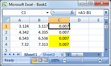
In Excel, we will start with a spreadsheet with two-value columns and a formula column. Column C, the formula column, uses conditional formatting that highlights the cells with a yellow color whenever they equal 0.007.
Conditional formatting allows the use of conditions such as cell value, formula, or functions to be used as an identifier for Excel to perform font changes, cell color changes, or other formatting changes.
You will notice in the following spreadsheet that cells C1 and C2 are not highlighted yellow, yet C3 and C4 are. However, the conditional formatting for C1:C4 are the same. If you subtract column A from column B on a calculator, you will find that the program is calculating the answer correctly.
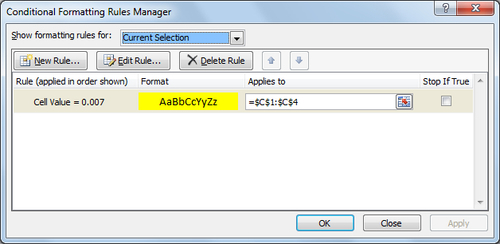
As noted earlier, conditional formatting utilizes conditions, as shown below. The condition set is that if the cell value equals 0.007, Excel should fill the cell with the yellow color.
You will need to change the formula to account for an absolute number of decimal places, specifically in this example, 3 decimal places.
Change the formula as shown and press Enter:
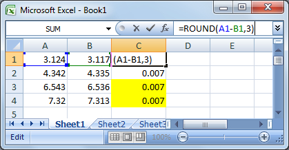
The reason for the difference is due to the method of storing and calculating numbers that Excel uses, it has to do with the concept of a floating decimal point and binary numbers. In short, due to the method in which Excel converts the numbers into memory, it reads the answer as 0.0069999999. By changing the formula to round the numbers to three decimal points, Excel changes the answer to .007 allowing the conditional formatting to recognize the answer as 0.007, and to match the answer that we received on the calculator.
When receiving Excel sheets from other sources, or when working with data, after using formulas to calculate data, it is often necessary to remove the formulas originally used. In order to remove the formulas, you could click on within each cell that contains a formula, and retype the answer hence removing the formula; however, this can become tedious.
In this recipe, you will learn how to quickly remove all formulas from a row of data retaining the calculated answers.
In the following example, column D contains the formula for calculating the profit from the wholesale price to retail price:
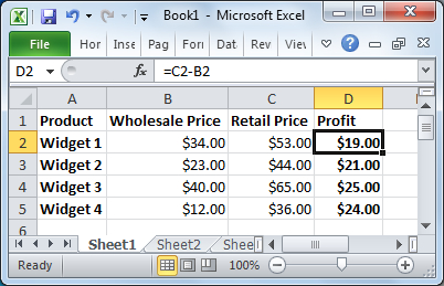
We will need to remove the formula used in column D while retaining the value data:

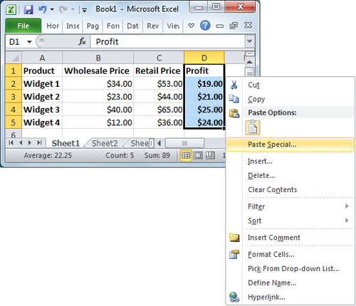
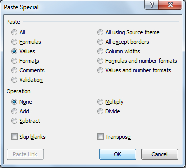
Using a regular copy and paste, Excel would by default copy the text, the formulas, and the formatting. By selecting paste special and only pasting values, Excel will remove all formulas and paste only the values from the formulas.
Many of the functions including Paste Special have shortcut buttons available within the Excel Ribbon. While the Excel Ribbon may offer some quicker access, utilizing the right-click menu provides an increased number of functions that are specific to your location within the Excel spreadsheet.
When working with large amounts of data, it can become difficult to locate blank spaces within the spreadsheet. Blank spaces can cause numerous issues including errors and breaks in formatting.
In this recipe, you will learn to locate and highlight all blanks within your data.
Smaller spreadsheets may allow you to quickly locate missed or blank information; however, Excel provides an automated method for performing this task that becomes increasingly more helpful with larger data-sets.
1. Under the Home tab click on the option Find & Select, and then choose Go To Special.

2. In the Go To Special... dialog box that opens, select the option for blank and click on OK.

3. All of the blanks within the data have now been highlighted.

4. Select a format for the blank cells, such as filling them with a color such as yellow. This now provides a contrasting visual indicator to locate blanks on the screen or when printed.

The Go To Special... option under Excel's built-in find feature provides several criteria that you can select to find data within your spreadsheet. By selecting blanks, Excel quickly parsed through the data and located and selected all the cells that contained no data. With all of the blank cells selected, you can easily apply a visual indicator.
While this recipe added a yellow fill to indicate blank cells, you can easily add other indicators such as lines, characters, and so on, which may provide for easier printing.
For further control of the formatting options used within this recipe, conditional formatting may provide a more automated, albeit, more involved method of locating and identifying blanks or other data. For more information on the use of conditional formatting, see the recipe Making printing easier to read.
When viewing large amounts of data on a computer screen it can be difficult to locate lines of data, especially when you need to scroll to the right; however, there are features that you can use such as freezing panes and highlighting. When printing, most of these options are not available.
In this recipe, you will learn how to utilize conditional formatting to add multi-colored bars to enhance visibility when printing Excel spreadsheets.
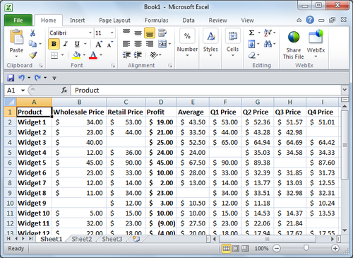
We will begin by selecting all of the values within the spreadsheet in order to apply formatting:
1. Select all rows and columns of the Excel spreadsheet, by clicking the box to the right of column A and above row 1, or utilizing the keyboard shortcut Ctrl + A.
2. From within the styles block on the ribbon located on the Home tab, select Conditional Formatting, and choose New Rule.
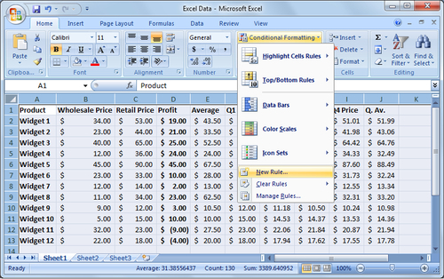
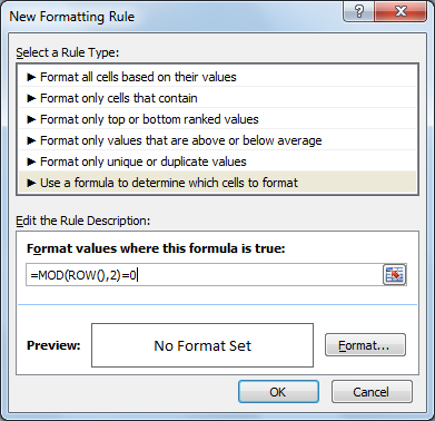
3. From the New Formatting Rule, select the option for Use a formula to determine which cells to format. In the provided formula box, type the formula as shown and select Format:
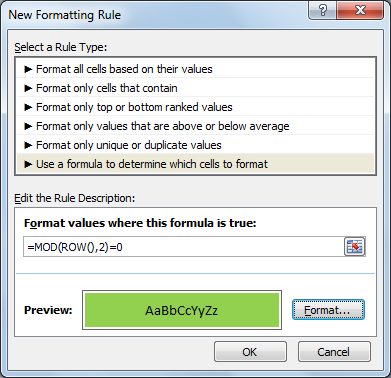
4. In format box, select the Fill tab, and choose a fill color such as green, and click on OK.
Tip
It is best to choose a lighter color that will not interfere with the readability of the text that it will be filling behind. Large financial documents printed on dot matrix style printers would commonly utilize either green or blue bar paper.

5. Select OK, to apply the conditional formatting from the New Formatting Rule window.
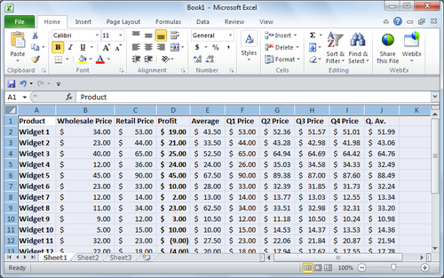
6. The Excel spreadsheet will now have alternating colored bars that when printed will provide a visual barrier to allow for easier viewing of wide rows of data.

The MOD function used in the conditional formatting rule returns the remainder after a number is divided by a divisor. For example, 5 divided by 3 would provide a remainder of 1.67, so =MOD(5,3) would also result in 1.67.
The ROW() function provides the number of the specific row. For instance, if you were to write the formula =ROW(A3), the result would be 3.
In the conditional formatting rule, only rows whose formula result is TRUE would be formatted. Because dividing by 2 would only present a 0 remainder in even numbered rows, the colored lines alternate to every other row providing the visual effect.
Financial data is compiled in numerous methods and from numerous sources. As discussed earlier, those sources do not always share the same methodology in how to format data. Also, when exporting data from many databases, the data is often forced together in long text strings. In most cases data that requires separation will contain some character or characteristic that will serve as the separation point.
This recipe will explain how to use identified separation points to split data into useable pieces.
As mentioned earlier within the recipe Setting up an Excel spreadsheet, the more granular the data you are working with, the more useful it will be. Long lines of text combining salesperson names and sales figures will make it impossible to perform automated function and arithmetic analysis.
The following data excerpt from quarterly sales figures combines all of the sales information into a single column as copied from a store register:
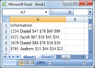
1. Highlight all of the data that needs to be split by selecting the column header. This will select the entire column allowing for the entire column of data to be split.
Note
During the splitting process, the data will be automatically entered into the adjacent cells. If the adjacent cells contain data, that data will be overwritten. If data is required adjacent to the data that needs to be split, you will need to insert several new columns to ensure that your adjacent information is not lost.
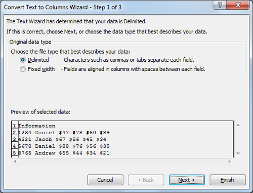
2. After highlighting column A, click on the Data tab from within the Excel ribbon and select Text to Columns.

3. The Text to Columns wizard will open. As noted earlier, data will often contain a natural separation point; in this case, that separation point is the space that separates the information. Make sure Delimited is selected and choose Next.
Tip
When there is a specific separation point such as a space, tab, period, colon, comma, or other character, the data is considered delimited. If no definable delimiter can be identified, a specific size or amount of characters may allow data separation, this is called fixed width.
4. In the list of delimiters, choose Space. Within the preview window, Excel will provide a preview of your data with vertical lines placed within the data. Each line signifies a new column, and how Excel will separate your data from the parameters you have selected. Choose Next.
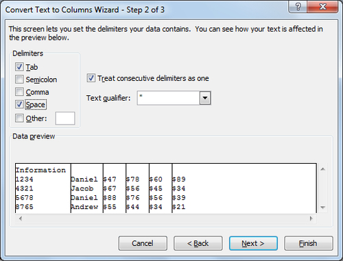
5. Excel will present you with formatting options for your data. After you have finished defining formatting, choose Finish.

The data has now been split and placed into adjacent columns.
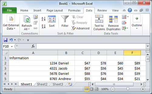
By specifying the delimiters, Excel was able to split your data and fill adjacent cells with the information. This separation now allows you to individually manipulate the data and utilize reporting and graphing functionality.
Now that the data has been split, it is important that you fill in labels for the data. While in some instances, reporting may require the data to be combined such as first and last name together, it is best to start with split data and individually determine which pieces of information to combine.
As we learned in earlier recipes, the best method for manipulating data in Excel is to break information into the smallest pieces possible. However, when porting this data to other locations or merging into reports, data may be better displayed by combining fields together; last name, middle initial, and first name for example. While smaller pieces are more efficiently manipulated, this broken form may not be read, when printed or communicated in reports, as easily.
In this recipe, you will learn how to combine a data field with textual characters to prepare data for review and reporting.
Combining data is a simple task that involves choosing the information that you wish to combine and adding any extra characters as needed. We will prepare the data below to be added to an employee timesheet. The full name field will need to display the employee number, last name, first name, and middle initial in the following form:
34567 — Doe, John F.
1. Begin by selecting an empty cell where the combined data is to be displayed:

2. Within the formula bar, type the following formula:

3. After pressing Enter, Cell A2 now displays the combined data. Click once again in cell A2, place your mouse over the small square that is displayed in the lower right-hand corner of the highlighting, and drag your mouse down to the last row that contains data; in this case row 4. Then release the mouse.

The formula entered used an ampersand (&), this symbol instructs Excel to combine information sequentially rather than attempting to add it together. By placing the hyphen (-), space ( ), comma (,), and period (.) in between quotation marks ("), Excel recognizes that the information is to be displayed as text. This combined with the ampersand combines the data within the cell references and quotations to build the new text string.
Excel has a built-in function for stringing data together called CONCATENATE. This formula allows textual strings to be listed sequentially without the use of an ampersand; however, the ampersand formula allows for greater flexibility and the inclusion of formula results within the combined string, whereas CONCATENATE treats all information as text.
As evidenced throughout the recipes so far, data may be received in varying formats, and may need to be changed prior to being sent elsewhere. This need for modification becomes increasingly important when sharing financial data internationally. Countries differ in method in which data is displayed, such as dates.
In this recipe, we will modify date information to display this and other information differently.
1. Select the column that contains the date to be modified by selecting the column header:

2. After the column has been selected, right-click on the column header and choose Format Cells:
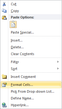
3. From the Format Cells window, select Date from the Category list. After Date has been selected, Excel will display the formatting methodology that it is used within the list:

In this case, Excel has determined that the formatting methodology used was *3/14/2001. The list of formatting options for dates as with many of the other categories contains a list of pre-formatted options; however, these options do not often contain all the necessary formatting options you may require.
4. From the category list, choose Custom.
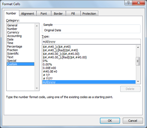
5. Highlight and remove the text displayed in the Type text field. Enter the following format, and then choose OK.

6. The data is now displayed in the format of 4-digit year, 2-digit month, and 2-digit day, separated by a period:

Normalizing data does not only involve modifying formats, it all also involves changing how the data is displayed on the screen. In financial reports, the data comprising the account total is extremely important; however, it may not always be beneficial to display all of the underlying information. You could remove the underlying transactions, but that would require a secondary sheet to view this data.
In this recipe, you will learn how to group data to display a summary line while hiding individual transactions; however, the transactions will remain as part of the original file and will be available for viewing at any time.
Before starting, it is important to layout the transaction details in a logical method. Financial statements work best with the summary line at the top of the transaction detail rather than below. We will begin with all summary information already included. For more information on adjusting the transaction summary, see the summary methods in Chapter 5's recipe, Better than a picture, graphically representing data without graphs.
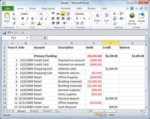
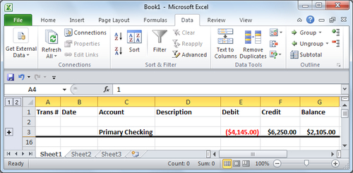
The following transaction details for "Primary Account" display individual transactions that display the balance for the account:
1. Beginning at the last line of data to be grouped for the individual account, highlight all of the rows of data stopping just under the summary row:

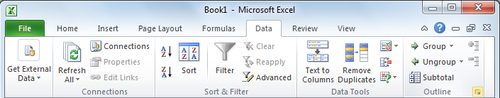
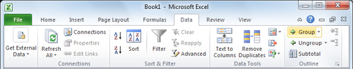
2. With the transaction detail highlighted, select the Data tab from the ribbon toolbar and click on the expansion icon on the lower right-hand corner of the Outline box:
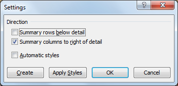
3. From the settings box that is displayed, uncheck the box for Summary rows below detail, and choose OK:
4. You will be returned to the highlighted data. The Data tab should still be selected. Choose the Group icon from the Outline box on the ribbon:
5. A grouping column will now appear on the far left side of the transaction data with a minus (-) sign in line with the summary row. Click the minus sign:
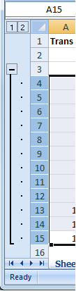
The transaction details have now been hidden leaving only the summary row. The transaction can be displayed at any time by clicking the plus (+) sign to the left of the summary row:
By deselecting the checkbox for displaying summary below data, Excel will allow the drill-down option above the data in-line with the summary row also located above the transaction details.
The outline functionality allows grouping of data to reduce the amount shown on the screen.
The outline function within Excel also contains summarization formulas including subtotal and average. These formulas can be added automatically.
When viewing financial summaries that utilize formulas, there are numerous reasons that you may need to view the formulas. In a sheet that utilizes many formulas, it may take a great deal of time to view each individual formula by selecting the cell and displaying the formula within the formula bar.
In this recipe, you will learn to display all the formulas within a sheet listed within the cell that contains a formula.
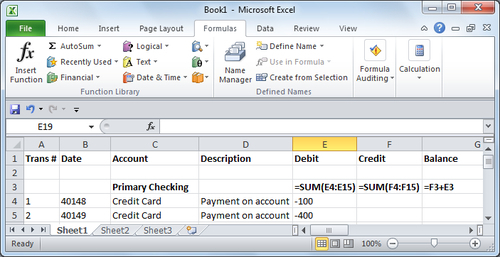
The following sheet contains a transaction register that utilizes formulas to provide a total of credit, debit, and remainder balances:
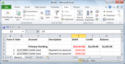
While displaying the active Excel sheet that contains formulas to be displayed, on your keyboard press Ctrl + ~ (tilde):
The Excel sheet now displays all of the formulas currently used. To turn off this display, simply press CTRL + ~ again.