Download code from GitHub
Getting Started with Time Series
In this chapter, we introduce the main concepts and techniques used in time series analysis. The chapter begins by defining time series and explaining why the analysis of these datasets is a relevant topic in data science. After that, we describe how to load time series data using the pandas library. The chapter dives into the basic components of a time series, such as trend and seasonality. One key concept of time series analysis covered in this chapter is that of stationarity. We will explore several methods to assess stationarity using statistical tests.
The following recipes will be covered in this chapter:
- Loading a time series using
pandas - Visualizing a time series
- Resampling a time series
- Dealing with missing values
- Decomposing a time series
- Computing autocorrelation
- Detecting stationarity
- Dealing with heteroskedasticity
- Loading and visualizing a multivariate time series
- Resampling a multivariate time series
- Analyzing the correlation among pairs of variables
By the end of this chapter, you will have a solid foundation in the main aspects of time series analysis. This includes loading and preprocessing time series data, identifying its basic components, decomposing time series, detecting stationarity, and expanding this understanding to a multivariate setting. This knowledge will serve as a building block for the subsequent chapters.
Technical requirements
To work through this chapter, you need to have Python 3.9 installed on your machine. We will work with the following libraries:
pandas(2.1.4)numpy(1.26.3)statsmodels(0.14.1)pmdarima(2.0.4)seaborn(0.13.2)
You can install these libraries using pip:
pip install pandas numpy statsmodels pmdarima seaborn
In our setup, we used pip version 23.3.1. The code for this chapter can be found at the following GitHub URL: https://github.com/PacktPublishing/Deep-Learning-for-Time-Series-Data-Cookbook
Loading a time series using pandas
In this first recipe, we start by loading a dataset in a Python session using pandas. Throughout this book, we’ll work with time series using pandas data structures. pandas is a useful Python package for data analysis and manipulation. Univariate time series can be structured as pandas Series objects, where the values of the series have an associated index or timestamp with a pandas.Index structure.
Getting ready
We will focus on a dataset related to solar radiation that was collected by the U.S. Department of Agriculture. The data, which contains information about solar radiation (in watts per square meter), spans from October 1, 2007, to October 1, 2013. It was collected at an hourly frequency totaling 52,608 observations.
You can download the dataset from the GitHub URL provided in the Technical requirements section of this chapter. You can also find the original source at the following URL: https://catalog.data.gov/dataset/data-from-weather-snow-and-streamflow-data-from-four-western-juniper-dominated-experimenta-b9e22.
How to do it…
The dataset is a .csv file. In pandas, we can load a .csv file using the pd.read_csv() function:
import pandas as pd
data = pd.read_csv('path/to/data.csv',
                   parse_dates=['Datetime'],
                   index_col='Datetime')
series = data['Incoming Solar']
In the preceding code, note the following:
- First, we import
pandasusing theimportkeyword. Importing this library is a necessary step to make its methods available in a Python session. - The main argument to
pd.read_csvis the file location. Theparse_datesargument automatically converts the input variables (in this case,Datetime) into a datetime format. Theindex_colargument sets the index of the data to theDatetimecolumn. - Finally, we subset the
dataobject using squared brackets to get theIncoming Solarcolumn, which contains the information about solar radiation at each time step.
How it works…
The following table shows a sample of the data. Each row represents the level of the time series at a particular hour.
|
Datetime |
Incoming Solar |
|
2007-10-01 09:00:00 |
35.4 |
|
2007-10-01 10:00:00 |
63.8 |
|
2007-10-01 11:00:00 |
99.4 |
|
2007-10-01 12:00:00 |
174.5 |
|
2007-10-01 13:00:00 |
157.9 |
|
2007-10-01 14:00:00 |
345.8 |
|
2007-10-01 15:00:00 |
329.8 |
|
2007-10-01 16:00:00 |
114.6 |
|
2007-10-01 17:00:00 |
29.9 |
|
2007-10-01 18:00:00 |
10.9 |
|
2007-10-01 19:00:00 |
0.0 |
Table 1.1: Sample of an hourly univariate time series
The series object that contains the time series is a pandas Series data structure. This structure contains several methods for time series analysis. We could also create a Series object by calling pd.Series with a dataset and the respective time series. The following is an example of this: pd.Series(data=values, index=timestamps), where values refers to the time series values and timestamps represents the respective timestamp of each observation.
Visualizing a time series
Now, we have a time series loaded in a Python session. This recipe walks you through the process of visualizing a time series in Python. Our goal is to create a line plot of the time series data, with the dates on the x axis and the value of the series on the y axis.
Getting ready
There are several data visualization libraries in Python. Visualizing a time series is useful to quickly identify patterns such as trends or seasonal effects. A graphic is an easy way to understand the dynamics of the data and to spot any anomalies within it.
In this recipe, we will create a time series plot using two different libraries: pandas and seaborn. seaborn is a popular data visualization Python library.
How to do it…
pandas Series objects contain a plot() method for visualizing time series. You can use it as follows:
series.plot(figsize=(12,6), title='Solar radiation time series')
The plot() method is called with two arguments. We use the figsize argument to change the size of the plot. In this case, we set the width and height of the figure to 12 and 6 inches, respectively. Another argument is title, which we set to Solar radiation time series. You can check the pandas documentation for a complete list of acceptable arguments.
You use it to plot a time series using seaborn as follows:
import matplotlib.pyplot as plt
import seaborn as sns
series_df = series.reset_index()
plt.rcParams['figure.figsize'] = [12, 6]
sns.set_theme(style='darkgrid')
sns.lineplot(data=series_df, x='Datetime', y='Incoming Solar')
plt.ylabel('Solar Radiation')
plt.xlabel('')
plt.title('Solar radiation time series')
plt.show()
plt.savefig('assets/time_series_plot.png')
The preceding code includes the following steps:
- Import
seabornandmatplotlib, two data visualization libraries. - Transform the time series into a
pandasDataFrame object by calling thereset_index()method. This step is required becauseseaborntakes DataFrame objects as the main input. - Configure the figure size using
plt.rcParamsto a width of 12 inches and a height of 6 inches. - Set the plot theme to
darkgridusing theset_theme()method. - Use the
lineplot()method to build the plot. Besides the input data, it takes the name of the column for each of the axes:DatetimeandIncoming Solarfor the x axis and y axis, respectively. - Configure the plot parameters, namely the y-axis label (
ylabel), x-axis label (xlabel), andtitle. - Finally, we use the
showmethod to display the plot andsavefigto store it as a.pngfile.
How it works…
The following figure shows the plot obtained from the seaborn library:
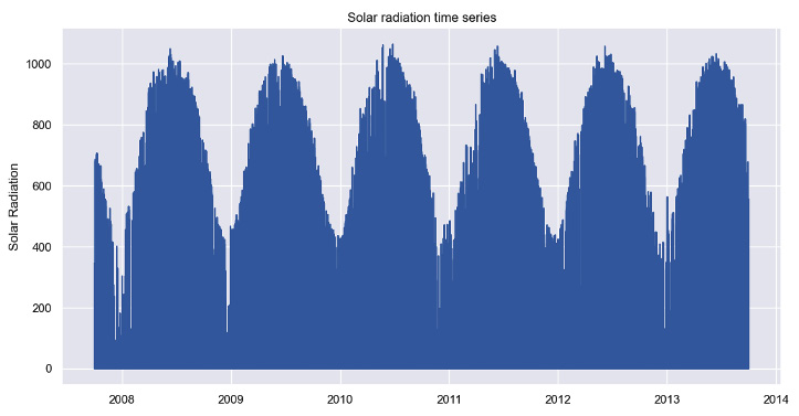
Figure 1.1: Time series plot using seaborn
The example time series shows a strong yearly seasonality, where the average level is lower at the start of the year. Apart from some fluctuations and seasonality, the long-term average level of the time series remains stable over time.
We learned about two ways of creating a time series plot. One uses the plot() method that is available in pandas, and another one uses seaborn, a Python library dedicated to data visualization. The first one provides a quick way of visualizing your data. But seaborn has a more powerful visualization toolkit that you can use to create beautiful plots.
There’s more…
The type of plot created in this recipe is called a line plot. Both pandas and seaborn can be used to create other types of plots. We encourage you to go through the documentation to learn about these.
Resampling a time series
Time series resampling is the process of changing the frequency of a time series, for example, from hourly to daily. This task is a common preprocessing step in time series analysis and this recipe shows how to do it with pandas.
Getting ready
Changing the frequency of a time series is a common preprocessing step before analysis. For example, the time series used in the preceding recipes has an hourly granularity. Yet, our goal may be to study daily variations. In such cases, we can resample the data into a different period. Resampling is also an effective way of handling irregular time series – those that are collected in irregularly spaced periods.
How to do it…
We’ll go over two different scenarios where resampling a time series may be useful: when changing the sampling frequency and when dealing with irregular time series.
The following code resamples the time series into a daily granularity:
series_daily = series.resample('D').sum() The daily granularity is specified with the input D to the resample () method. The values of each corresponding day are summed together using the sum() method.
Most time series analysis methods work under the assumption that the time series is regular; in other words, it is collected in regularly spaced time intervals (for example, every day). But some time series are naturally irregular. For instance, the sales of a retail product occur at arbitrary timestamps as customers arrive at a store.
Let us simulate sale events with the following code:
import numpy as np
import pandas as pd
n_sales = 1000
start = pd.Timestamp('2023-01-01 09:00')
end = pd.Timestamp('2023-04-01')
n_days = (end – start).days + 1
irregular_series = pd.to_timedelta(np.random.rand(n_sales) * n_days,
                                   unit='D') + start
The preceding code creates 1000 sale events from 2023-01-01 09:00 to 2023-04-01. A sample of this series is shown in the following table:
|
ID |
Timestamp |
|
1 |
2023-01-01 15:18:10 |
|
2 |
2023-01-01 15:28:15 |
|
3 |
2023-01-01 16:31:57 |
|
4 |
2023-01-01 16:52:29 |
|
5 |
2023-01-01 23:01:24 |
|
6 |
2023-01-01 23:44:39 |
Table 1.2: Sample of an irregular time series
Irregular time series can be transformed into a regular frequency by resampling. In the case of sales, we will count how many sales occurred each day:
ts_sales = pd.Series(0, index=irregular_series)
tot_sales = ts_sales.resample('D').count()
First, we create a time series of zeros based on the irregular timestamps (ts_sales). Then, we resample this dataset into a daily frequency (D) and use the count() method to count how many observations occur each day. The tot_sales reconstructed time series can be used for other tasks, such as forecasting daily sales.
How it works…
A sample of the reconstructed time series concerning solar radiation is shown in the following table:
|
Datetime |
Incoming Solar |
|
2007-10-01 |
1381.5 |
|
2007-10-02 |
3953.2 |
|
2007-10-03 |
3098.1 |
|
2007-10-04 |
2213.9 |
Table 1.3: Solar radiation time series after resampling
Resampling is a cornerstone preprocessing step in time series analysis. This technique can be used to change a time series into a different granularity or to convert an irregular time series into a regular one.
The summary statistic is an important input to consider. In the first case, we used sum to add the hourly solar radiation values observed each day. In the case of the irregular time series, we used the count() method to count how many events occurred in each period. Yet, you can use other summary statistics according to your needs. For example, using the mean would take the average value of each period to resample the time series.
There’s more…
We resampled to daily granularity. A list of available options is available here: https://pandas.pydata.org/docs/user_guide/timeseries.html#dateoffset-objects.
Dealing with missing values
In this recipe, we’ll cover how to impute time series missing values. We’ll discuss different methods of imputing missing values and the factors to consider when choosing a method. We’ll show an example of how to solve this problem using pandas.
Getting ready
Missing values are an issue that plagues all kinds of data, including time series. Observations are often unavailable for various reasons, such as sensor failure or annotation errors. In such cases, data imputation can be used to overcome this problem. Data imputation works by assigning a value based on some rule, such as the mean or some predefined value.
How to do it…
We start by simulating missing data. The following code removes 60% of observations from a sample of two years of the solar radiation time series:
import numpy as np
sample_with_nan = series_daily.head(365 * 2).copy()
size_na=int(0.6 * len(sample_with_nan))
idx = np.random.choice(a=range(len(sample_with_nan)),
                       size=size_na,
                       replace=False)
sample_with_nan[idx] = np.nan
We leverage the np.random.choice() method from numpy to select a random sample of the time series. The observations of this sample are changed to a missing value (np.nan).
In datasets without temporal order, it is common to impute missing values using central statistics such as the mean or median. This can be done as follows:
average_value = sample_with_nan.mean()
imp_mean = sample_with_nan.fillna(average_value)
Time series imputation must take into account the temporal nature of observations. This means that the assigned value should follow the dynamics of the series. A more common approach in time series is to impute missing data with the last known observation. This approach is implemented in the ffill() method:
imp_ffill = sample_with_nan.ffill()
Another, less common, approach that uses the order of observations is bfill():
imp_bfill = sample_with_nan.bfill()
The bfill() method imputes missing data with the next available observation in the dataset.
How it works…
The following figure shows the reconstructed time series after imputation with each method:
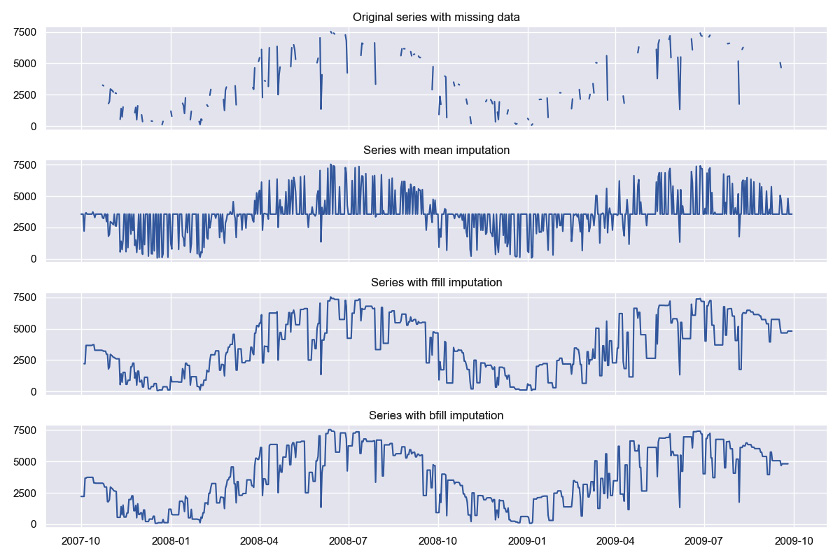
Figure 1.2: Imputing missing data with different strategies
The mean imputation approach misses the time series dynamics, while both ffill and bfill lead to a reconstructed time series with similar dynamics as the original time series. Usually, ffill is preferable because it does not break the temporal order of observations, that is, using future information to alter (impute) the past.
There’s more…
The imputation process can also be carried out using some conditions, such as limiting the number of imputed observations. You can learn more about this in the documentation pages of these functions, for example, https://pandas.pydata.org/docs/reference/api/pandas.DataFrame.ffill.html.
Decomposing a time series
Time series decomposition is the process of splitting a time series into its basic components, such as trend or seasonality. This recipe explores different techniques to solve this task and how to choose among them.
Getting ready
A time series is composed of three parts – trend, seasonality, and the remainder:
- The trend characterizes the long-term change in the level of a time series. Trends can be upward (increase in level) or downward (decrease in level), and they can also change over time.
- Seasonality refers to regular variations in fixed periods, such as every day. The solar radiation time series plotted in the preceding recipe shows a clear yearly seasonality. Solar radiation is higher during summer and lower during winter.
- The remainder (also called irregular) of the time series is what is left after removing the trend and seasonal components.
Breaking a time series into its components is useful to understand the underlying structure of the data.
We’ll describe the process of time series decomposition with two methods: the classical decomposition approach and a method based on local regression. You’ll also learn how to extend the latter method to time series with multiple seasonal patterns.
How to do it…
There are several approaches for decomposing a time series into its basic parts. The simplest method is known as classical decomposition. This approach is implemented in the statsmodels library and can be used as follows:
from statsmodels.tsa.seasonal import seasonal_decompose
result = seasonal_decompose(x=series_daily,
                            model='additive',
                            period=365)
Besides the dataset, you need to specify the period and the type of model. For a daily time series with a yearly seasonality, the period should be set to 365, which is the number of days in a year. The model parameter can be either additive or multiplicative. We’ll go into more detail about this in the next section.
Each component is stored as an attribute of the results in an object:
result.trend
result.seasonal
result.resid
Each of these attributes returns a time series with the respective component.
Arguably, one of the most popular methods for time series decomposition is STL (which stands for Seasonal and Trend decomposition using LOESS). This method is also available on statsmodels:
from statsmodels.tsa.seasonal import STL
result = STL(endog=series_daily, period=365).fit()
In the case of STL, you don’t need to specify a model as we did with the classical method.
Usually, time series decomposition approaches work under the assumption that the dataset contains a single seasonal pattern. Yet, time series collected in high sampling frequencies (such as hourly or daily) can contain multiple seasonal patterns. For example, an hourly time series can show both regular daily and weekly variations.
The MSTL() method (short for Multiple STL) extends MSTL for time series with multiple seasonal patterns. You can specify the period for each seasonal pattern in a tuple as the input for the period argument. An example is shown in the following code:
from statsmodels.tsa.seasonal import MSTL
result = MSTL(endog=series_daily, periods=(7, 365)).fit()
In the preceding code, we passed two periods as input: 7 and 365. These periods attempt to capture weekly and yearly seasonality in a daily time series.
How it works…
In a given time step i, the value of the time series (Yi) can be decomposed using an additive model, as follows:
Yi = Trendi+Seasonalityi+Remainderi
This decomposition can also be multiplicative:
Yi = Trendi×Seasonalityi×Remainderi
The most appropriate approach, additive or multiplicative, depends on the input data. But you can turn a multiplicative decomposition into an additive one by transforming the data with the logarithm function. The logarithm stabilizes the variance, thus making the series additive regarding its components.
The results of the classical decomposition are shown in the following figure:

Figure 1.3: Time series components after decomposition with the classical method
In the classical decomposition, the trend is estimated using a moving average, for example, the average of the last 24 hours (for hourly series). Seasonality is estimated by averaging the values of each period. STL is a more flexible method for decomposing a time series. It can handle complex patterns, such as irregular trends or outliers. STL leverages LOESS, which stands for locally weighted scatterplot smoothing, to extract each component.
There’s more…
Decomposition is usually done for data exploration purposes. But it can also be used as a preprocessing step for forecasting. For example, some studies show that removing seasonality before training a neural network improves forecasting performance.
See also
You can learn more about this in the following references:
- Hewamalage, Hansika, Christoph Bergmeir, and Kasun Bandara. “Recurrent neural networks for time series forecasting: Current status and future directions.” International Journal of Forecasting 37.1 (2021): 388-427.
- Hyndman, Rob J., and George Athanasopoulos. Forecasting: Principles and Practice. OTexts, 2018.
Computing autocorrelation
This recipe guides you through the process of computing autocorrelation. Autocorrelation is a measure of the correlation between a time series and itself at different lags, and it is helpful to understand the structure of time series, specifically, to quantify how past values affect the future.
Getting ready
Correlation is a statistic that measures the linear relationship between two random variables. Autocorrelation extends this notion to time series data. In time series, the value observed in a given time step will be similar to the values observed before it. The autocorrelation function quantifies the linear relationship between a time series and a lagged version of itself. A lagged time series refers to a time series that is shifted over a number of periods.
How to do it…
We can compute the autocorrelation function using statsmodels:
from statsmodels.tsa.stattools import acf
acf_scores = acf(x=series_daily, nlags=365)
The inputs to the function are a time series and the number of lags to analyze. In this case, we compute autocorrelation up to 365 lags, a full year of data.
We can also use statsmodels to compute the partial autocorrelation function. This measure extends the autocorrelation by controlling for the correlation of the time series at shorter lags:
from statsmodels.tsa.stattools import pacf
pacf_scores = pacf(x=series_daily, nlags=365)
The statsmodels library also provides functions to plot the results of autocorrelation analysis:
from statsmodels.graphics.tsaplots import plot_acf, plot_pacf
plot_acf(series_daily, lags=365)
plot_pacf(series_daily, lags=365)
How it works…
The following figure shows the autocorrelation of the daily solar radiation time series up to 365 lags.
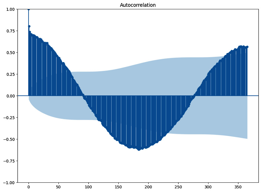
Figure 1.4: Autocorrelation scores up to 365 lags. The oscillations indicate seasonality
The oscillations in this plot are due to the yearly seasonal pattern. The analysis of autocorrelation is a useful approach to detecting seasonality.
There’s more…
The autocorrelation at each seasonal lag is usually large and positive. Besides, sometimes autocorrelation decays slowly along the lags, which indicates the presence of a trend. You can learn more about this from the following URL: https://otexts.com/fpp3/components.html.
The partial autocorrelation function is an important tool for identifying the order of autoregressive models. The idea is to select the number of lags whose partial autocorrelation is significant.
Detecting stationarity
Stationarity is a central concept in time series analysis and an important assumption made by many time series models. This recipe walks you through the process of testing a time series for stationarity.
Getting ready
A time series is stationary if its statistical properties do not change. It does not mean that the series does not change over time, just that the way it changes does not itself change over time. This includes the level of the time series, which is constant under stationary conditions. Time series patterns such as trend or seasonality break stationarity. Therefore, it may help to deal with these issues before modeling. As we described in the Decomposing a time series recipe, there is evidence that removing seasonality improves the forecasts of deep learning models.
We can stabilize the mean level of the time series by differencing. Differencing is the process of taking the difference between consecutive observations. This process works in two steps:
- Estimate the number of differencing steps required for stationarity.
- Apply the required number of differencing operations.
How to do it…
We can estimate the required differencing steps with statistical tests, such as the augmented Dickey-Fuller test, or the KPSS test. These are implemented in the ndiffs() function, which is available in the pmdarima library:
from pmdarima.arima import ndiffs
ndiffs(x=series_daily, test='adf')
Besides the time series, we pass test='adf' as an input to set the method to the augmented Dickey-Fuller test. The output of this function is the number of differencing steps, which in this case is 1. Then, we can differentiate the time series using the diff() method:
series_changes = series_daily.diff()
Differencing can also be applied over seasonal periods. In such cases, seasonal differencing involves computing the difference between consecutive observations of the same seasonal period:
from pmdarima.arima import nsdiffs
nsdiffs(x=series_changes, test='ch', m=365)
Besides the data and the test (ch for Canova-Hansen), we also specify the number of periods. In this case, this parameter is set to 365 (number of days in a year).
How it works…
The differenced time series is shown in the following figure.
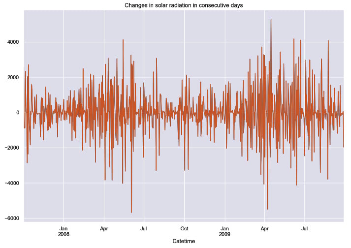
Figure 1.5: Sample of the series of changes between consecutive periods after differencing
Differencing works as a preprocessing step. First, the time series is differenced until it becomes stationary. Then, a forecasting model is created based on the differenced time series. The forecasts provided by the model can be transformed to the original scale by reverting the differencing operations.
There’s more…
In this recipe, we focused on two particular methods for testing stationarity. You can check other options in the function documentation: https://alkaline-ml.com/pmdarima/modules/generated/pmdarima.arima.ndiffs.html.
Dealing with heteroskedasticity
In this recipe, we delve into the variance of time series. The variance of a time series is a measure of how spread out the data is and how this dispersion evolves over time. You’ll learn how to handle data with a changing variance.
Getting ready
The variance of time series can change over time, which also violates stationarity. In such cases, the time series is referred to as heteroskedastic and usually shows a long-tailed distribution. This means the data is left- or right-skewed. This condition is problematic because it impacts the training of neural networks and other models.
How to do it…
Dealing with non-constant variance is a two-step process. First, we use statistical tests to check whether a time series is heteroskedastic. Then, we use transformations such as the logarithm to stabilize the variance.
We can detect heteroskedasticity using statistical tests such as the White test or the Breusch-Pagan test. The following code implements these tests based on the statsmodels library:
import statsmodels.stats.api as sms
from statsmodels.formula.api import ols
series_df = series_daily.reset_index(drop=True).reset_index()
series_df.columns = ['time', 'value']
series_df['time'] += 1
olsr = ols('value ~ time', series_df).fit()
_, pval_white, _, _ = sms.het_white(olsr.resid, olsr.model.exog)
_, pval_bp, _, _ = sms.het_breuschpagan(olsr.resid, olsr.model.exog)
The preceding code follows these steps:
- Import the
statsmodelsmodulesolsandstats. - Create a DataFrame based on the values of the time series and the row they were collected at (
1for the first observation). - Create a linear model that relates the values of the time series with the
timecolumn. - Run
het_white(White) andhet_breuschpagan(Breusch-Pagan) to apply the variance tests.
The output of the tests is a p-value, where the null hypothesis posits that the time series has constant variance. So, if the p-value is below the significance value, we reject the null hypothesis and assume heteroskedasticity.
The simplest way to deal with non-constant variance is by transforming the data using the logarithm. This operation can be implemented as follows:
import numpy as np
class LogTransformation:
    @staticmethod
    def transform(x):
        xt = np.sign(x) * np.log(np.abs(x) + 1)
        return xt
    @staticmethod
    def inverse_transform(xt):
        x = np.sign(xt) * (np.exp(np.abs(xt)) - 1)
        return x
The preceding code is a Python class called LogTransformation. It contains two methods: transform() and inverse_transform(). The first transforms the data using the logarithm and the second reverts that operation.
We apply the transform() method to the time series as follows:
series_log = LogTransformation.transform(series_daily)
The log is a particular case of Box-Cox transformation that is available in the scipy library. You can implement this method as follows:
series_transformed, lmbda = stats.boxcox(series_daily)
The stats.boxcox() method estimates a transformation parameter, lmbda, which can be used to revert the operation.
How it works…
The transformations outlined in this recipe stabilize the variance of a time series. They also bring the data distribution closer to the Normal distribution. These transformations are especially useful for neural networks as they help avoid saturation areas. In neural networks, saturation occurs when the model becomes insensitive to different inputs, thus compromising the training process.
There’s more…
The Yeo-Johnson power transformation is similar to the Box-Cox transformation but allows for negative values in the time series. You can learn more about this method with the following link: https://docs.scipy.org/doc/scipy/reference/generated/scipy.stats.yeojohnson.html.
See also
You can learn more about the importance of the logarithm transformation in the following reference:
Bandara, Kasun, Christoph Bergmeir, and Slawek Smyl. “Forecasting across time series databases using recurrent neural networks on groups of similar series: A clustering approach.” Expert Systems with Applications 140 (2020): 112896.
Loading and visualizing a multivariate time series
So far, we’ve learned how to analyze univariate time series. Yet, multivariate time series are also relevant in real-world problems. This recipe explores how to load a multivariate time series. Before, we used the pandas Series structure to handle univariate time series. Multivariate time series are better structured as pandas DataFrame objects.
Getting ready
A multivariate time series contains multiple variables. The concepts underlying time series analysis are extended to cases where multiple variables evolve over time and are interrelated with each other. The relationship between the different variables can be difficult to model, especially when the number of these variables is large.
In many real-world applications, multiple variables can influence each other and exhibit a temporal dependency. For example, in weather modeling, the incoming solar radiation is correlated with other meteorological variables, such as air temperature or humidity. Considering these variables with a single multivariate model can be fundamental for modeling the dynamics of the data and getting better predictions.
We’ll continue to study the solar radiation dataset. This time series is extended by including extra meteorological information.
How to do it…
We’ll start by reading a multivariate time series. Like in the Loading a time series using pandas recipe, we resort to pandas and read a .csv file into a DataFrame data structure:
import pandas as pd
data = pd.read_csv('path/to/multivariate_ts.csv',
                   parse_dates=['datetime'],
                   index_col='datetime')
The parse_dates and index_col arguments ensure that the index of the DataFrame is a DatetimeIndex object. This is important so that pandas treats this object as a time series. After loading the time series, we can transform and visualize it using the plot() method:
data_log = LogTransformation.transform(data)
sample = data_log.tail(1000)
mv_plot = sample.plot(figsize=(15, 8),
                      title='Multivariate time series',
                      xlabel='',
                      ylabel='Value')
mv_plot.legend(fancybox=True, framealpha=1)
The preceding code follows these steps:
- First, we transform the data using the logarithm.
- We take the last 1,000 observations to make the visualization less cluttered.
- Finally, we use the
plot()method to create a visualization. We also calllegendto configure the legend of the plot.
How it works…
A sample of the multivariate time series is displayed in the following figure:
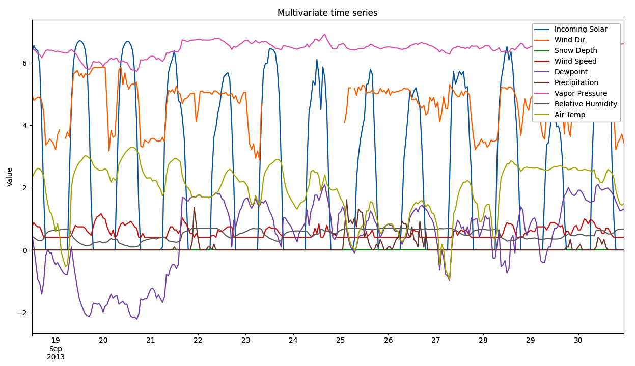
Figure 1.6: Multivariate time series plot
The process of loading a multivariate time series works like the univariate case. The main difference is that a multivariate time series is stored in Python as a DataFrame object rather than a Series one.
From the preceding plot, we can notice that different variables follow different distributions and have distinct average and dispersion levels.
Resampling a multivariate time series
This recipe revisits the topic of resampling but focuses on multivariate time series. We’ll explain why resampling can be a bit tricky for multivariate time series due to the eventual need to use distinct summary statistics for different variables.
Getting ready
When resampling a multivariate time, you may need to apply different summary statistics depending on the variable. For example, you may want to sum up the solar radiation observed at each hour to get a sense of how much power you could generate. Yet, taking the average, instead of the sum, is more sensible when summarizing wind speed because this variable is not cumulative.
How to do it…
We can pass a Python dictionary that details which statistic should be applied to each variable. Then, we can pass this dictionary to the agg () method, as follows:
stat_by_variable = {
    'Incoming Solar': 'sum',
    'Wind Dir': 'mean',
    'Snow Depth': 'sum',
    'Wind Speed': 'mean',
    'Dewpoint': 'mean',
    'Precipitation': 'sum',
    'Vapor Pressure': 'mean',
    'Relative Humidity': 'mean',
    'Air Temp': 'max',
}
data_daily = data.resample('D').agg(stat_by_variable)
We aggregate the time series into a daily periodicity using different summary statistics. For example, we want to sum up the solar radiation observed each day. For the air temperature variable (Air Temp), we take the maximum value observed each day.
How it works…
By using a dictionary to pass different summary statistics, we can adjust the frequency of the time series in a more flexible way. Note that if you wanted to apply the mean for all variables, you would not need a dictionary. A simpler way would be to run data.resample('D').mean().
Analyzing correlation among pairs of variables
This recipe walks you through the process of using correlation to analyze a multivariate time series. This task is useful to understand the relationship among the different variables in the series and thereby understand its dynamics.
Getting ready
A common way to analyze the dynamics of multiple variables is by computing the correlation of each pair. You can use this information to perform feature selection. For example, when pairs of variables are highly correlated, you may want to keep only one of them.
How to do it…
First, we compute the correlation among each pair of variables:
corr_matrix = data_daily.corr(method='pearson')
We can visualize the results using a heatmap from the seaborn library:
import seaborn as sns
import matplotlib.pyplot as plt
sns.heatmap(data=corr_matrix,
            cmap=sns.diverging_palette(230, 20, as_cmap=True),
            xticklabels=data_daily.columns,
            yticklabels=data_daily.columns,
            center=0,
            square=True,
            linewidths=.5,
            cbar_kws={"shrink": .5})
plt.xticks(rotation=30)
Heatmaps are a common way of visualizing matrices. We pick a diverging color set from sns.diverging_palette to distinguish between negative correlation (blue) and positive correlation (red).
How it works…
The following figure shows the heatmap with the correlation results:

Figure 1.7: Correlation matrix for a multivariate time series
The corr() method computes the correlation among each pair of variables in the data_daily object. In this case, we use the Pearson correlation with the method='pearson' argument. Kendall and Spearman are two common alternatives to the Pearson correlation.