The nearest neighbor algorithm classifies a data instance based on its neighbors. The class of a data instance determined by the k-nearest neighbor algorithm is the class with the highest representation among the k-closest neighbors.

In this chapter, we will cover the basics of the k-NN algorithm - understanding it and its implementation with a simple example: Mary and her temperature preferences. On the example map of Italy, you will learn how to choose a correct value k so that the algorithm can perform correctly and with the highest accuracy. You will learn how to rescale the values and prepare them for the k-NN algorithm with the example of house preferences. In the example of text classification, you will learn how to choose a good metric to measure the distances between the data points, and also how to eliminate the irrelevant dimensions in higher-dimensional space to ensure that the algorithm performs accurately.

As an example, if we know that our friend Mary feels cold when it is 10 degrees Celsius, but warm when it is 25 degrees Celsius, then in a room where it is 22 degrees Celsius, the nearest neighbor algorithm would guess that our friend would feel warm, because 22 is closer to 25 than to 10.

Suppose we would like to know when Mary feels warm and when she feels cold, as in the previous example, but in addition, wind speed data is also available when Mary was asked if she felt warm or cold:

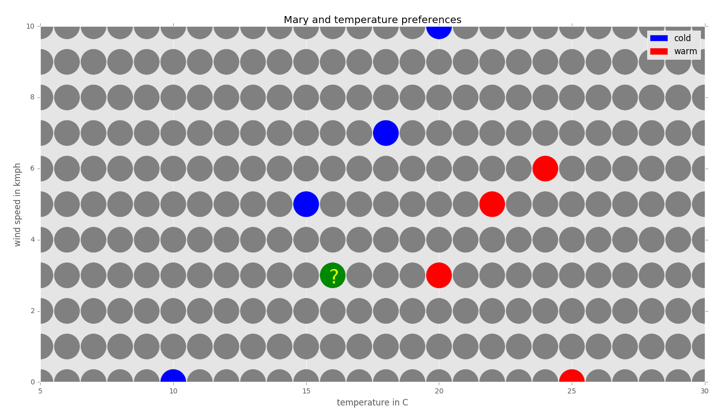
We could represent the data in a graph, as follows:

Now, suppose we would like to find out how Mary feels at the temperature 16 degrees Celsius with a wind speed of 3km/h using the 1-NN algorithm:

For simplicity, we will use a Manhattan metric to measure the distance between the neighbors on the grid. The Manhattan distance d_Man of a neighbor N₁=(x₁,y₁) from the neighbor N₂=(x₂,y₂) is defined to be d_Man=|x₁- x₂|+|y₁- y₂|.

Let us label the grid with distances around the neighbors to see which neighbor with a known class is closest to the point we would like to classify:

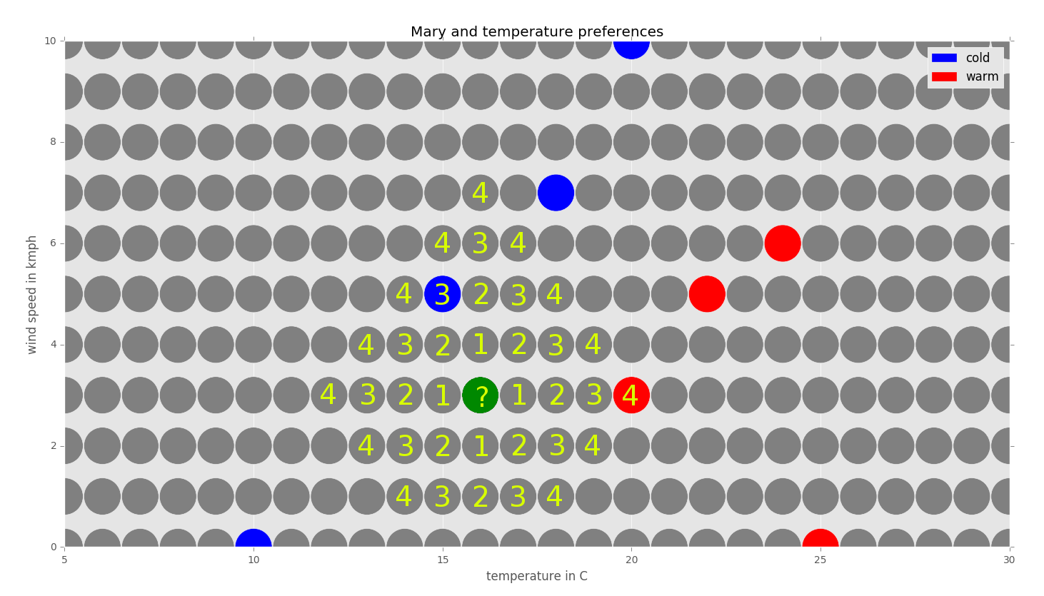
We can see that the closest neighbor with a known class is the one with the temperature 15 (blue) degrees Celsius and the wind speed 5km/h. Its distance from the questioned point is three units. Its class is blue (cold). The closest red (warm) neighbor is distanced four units from the questioned point. Since we are using the 1-nearest neighbor algorithm, we just look at the closest neighbor and, therefore, the class of the questioned point should be blue (cold).

By applying this procedure to every data point, we can complete the graph as follows:

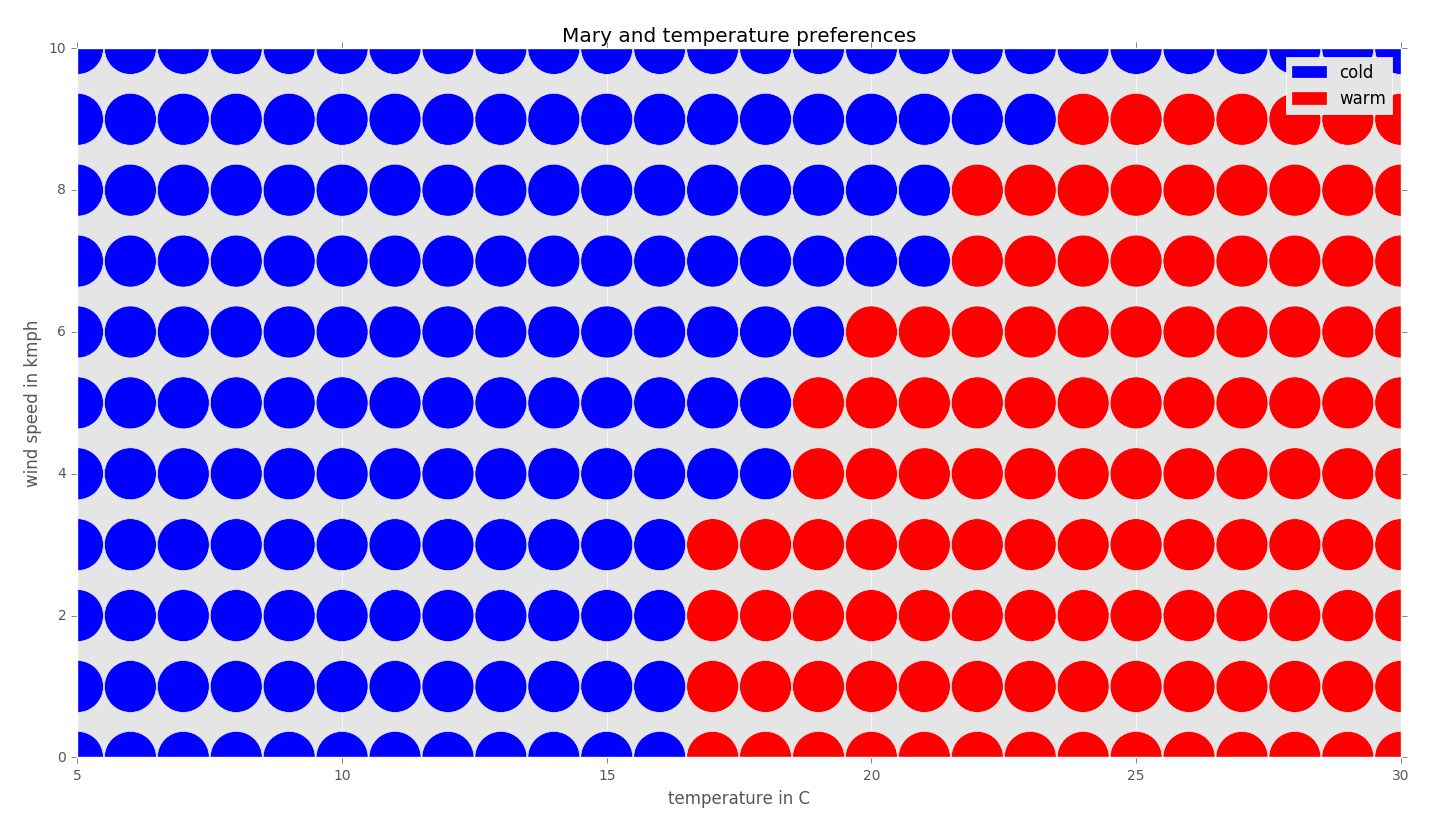
Note that sometimes a data point can be distanced from two known classes with the same distance: for example, 20 degrees Celsius and 6km/h. In such situations, we could prefer one class over the other or ignore these boundary cases. The actual result depends on the specific implementation of an algorithm.

We implement the k-NN algorithm in Python to find Mary's temperature preference. In the end of this section we also implement the visualization of the data produced in example Mary and her temperature preferences by the k-NN algorithm. The full compilable code with the input files can be found in the source code provided with this book. The most important parts are extracted here:

# source_code/1/mary_and_temperature_preferences/knn_to_data.py
# Applies the knn algorithm to the input data.
# The input text file is assumed to be of the format with one line per
# every data entry consisting of the temperature in degrees Celsius,
# wind speed and then the classification cold/warm.

import sys
sys.path.append('..')
sys.path.append('../../common')
import knn # noqa
import common # noqa

# Program start
# E.g. "mary_and_temperature_preferences.data"
input_file = sys.argv[1]
# E.g. "mary_and_temperature_preferences_completed.data"
output_file = sys.argv[2]
k = int(sys.argv[3])
x_from = int(sys.argv[4])
x_to = int(sys.argv[5])
y_from = int(sys.argv[6])
y_to = int(sys.argv[7])

data = common.load_3row_data_to_dic(input_file)
new_data = knn.knn_to_2d_data(data, x_from, x_to, y_from, y_to, k)
common.save_3row_data_from_dic(output_file, new_data)
# source_code/common/common.py
# ***Library with common routines and functions***
def dic_inc(dic, key):
    if key is None:
        pass
    if dic.get(key, None) is None:
        dic[key] = 1
    else:
        dic[key] = dic[key] + 1

# source_code/1/knn.py
# ***Library implementing knn algorihtm***

def info_reset(info):
    info['nbhd_count'] = 0
    info['class_count'] = {}

# Find the class of a neighbor with the coordinates x,y.
# If the class is known count that neighbor.
def info_add(info, data, x, y):
    group = data.get((x, y), None)
    common.dic_inc(info['class_count'], group)
    info['nbhd_count'] += int(group is not None)

# Apply knn algorithm to the 2d data using the k-nearest neighbors with
# the Manhattan distance.
# The dictionary data comes in the form with keys being 2d coordinates
# and the values being the class.
# x,y are integer coordinates for the 2d data with the range
# [x_from,x_to] x [y_from,y_to].
def knn_to_2d_data(data, x_from, x_to, y_from, y_to, k):
    new_data = {}
    info = {}
    # Go through every point in an integer coordinate system.
    for y in range(y_from, y_to + 1):
        for x in range(x_from, x_to + 1):
            info_reset(info)
            # Count the number of neighbors for each class group for
            # every distance dist starting at 0 until at least k
            # neighbors with known classes are found.
            for dist in range(0, x_to - x_from + y_to - y_from):
                # Count all neighbors that are distanced dist from
                # the point [x,y].
                if dist == 0:
                    info_add(info, data, x, y)
                else:
                    for i in range(0, dist + 1):
                        info_add(info, data, x - i, y + dist - i)
                        info_add(info, data, x + dist - i, y - i)
                    for i in range(1, dist):
                        info_add(info, data, x + i, y + dist - i)
                        info_add(info, data, x - dist + i, y - i)
                # There could be more than k-closest neighbors if the
                # distance of more of them is the same from the point
                # [x,y]. But immediately when we have at least k of
                # them, we break from the loop.
                if info['nbhd_count'] >= k:
                    break
            class_max_count = None
            # Choose the class with the highest count of the neighbors
            # from among the k-closest neighbors.
            for group, count in info['class_count'].items():
                if group is not None and (class_max_count is None or
                   count > info['class_count'][class_max_count]):
                    class_max_count = group
            new_data[x, y] = class_max_count
    return new_data

Input:

The program above will use the file below as the source of the input data. The file contains the table with the known data about Mary's temperature preferences:

# source_code/1/mary_and_temperature_preferences/
marry_and_temperature_preferences.data
10 0 cold
25 0 warm
15 5 cold
20 3 warm
18 7 cold
20 10 cold
22 5 warm
24 6 warm

Output:

We run the implementation above on the input file mary_and_temperature_preferences.data using the k-NN algorithm for k=1 neighbors. The algorithm classifies all the points with the integer coordinates in the rectangle with a size of (30-5=25) by (10-0=10), so with the a of (25+1) * (10+1) = 286 integer points (adding one to count points on boundaries). Using the wc command, we find out that the output file contains exactly 286 lines - one data item per point. Using the head command, we display the first 10 lines from the output file. We visualize all the data from the output file in the next section:

$ python knn_to_data.py mary_and_temperature_preferences.data mary_and_temperature_preferences_completed.data 1 5 30 0 10

$ wc -l mary_and_temperature_preferences_completed.data 
286 mary_and_temperature_preferences_completed.data

$ head -10 mary_and_temperature_preferences_completed.data 
7 3 cold
6 9 cold
12 1 cold
16 6 cold
16 9 cold
14 4 cold
13 4 cold
19 4 warm
18 4 cold
15 1 cold

Visualization:

For the visualization depicted earlier in this chapter, the matplotlib library was used. A data file is loaded, and then displayed in a scattered diagram:

# source_code/common/common.py
# returns a dictionary of 3 lists: 1st with x coordinates,
# 2nd with y coordinates, 3rd with colors with numeric values
def get_x_y_colors(data):
    dic = {}
    dic['x'] = [0] * len(data)
    dic['y'] = [0] * len(data)
    dic['colors'] = [0] * len(data)
    for i in range(0, len(data)):
        dic['x'][i] = data[i][0]
        dic['y'][i] = data[i][1]
        dic['colors'][i] = data[i][2]
    return dic
# source_code/1/mary_and_temperature_preferences/
mary_and_temperature_preferences_draw_graph.py 
import sys
sys.path.append('../../common')  # noqa
import common
import numpy as np
import matplotlib.pyplot as plt
import matplotlib.patches as mpatches
import matplotlib
matplotlib.style.use('ggplot')

data_file_name = 'mary_and_temperature_preferences_completed.data'
temp_from = 5
temp_to = 30
wind_from = 0
wind_to = 10

data = np.loadtxt(open(data_file_name, 'r'),
                  dtype={'names': ('temperature', 'wind', 'perception'),
                         'formats': ('i4', 'i4', 'S4')})

# Convert the classes to the colors to be displayed in a diagram.
for i in range(0, len(data)):
    if data[i][2] == 'cold':
        data[i][2] = 'blue'
    elif data[i][2] == 'warm':
        data[i][2] = 'red'
    else:
        data[i][2] = 'gray'
# Convert the array into the format ready for drawing functions.
data_processed = common.get_x_y_colors(data)

# Draw the graph.
plt.title('Mary and temperature preferences')
plt.xlabel('temperature in C')
plt.ylabel('wind speed in kmph')
plt.axis([temp_from, temp_to, wind_from, wind_to])
# Add legends to the graph.
blue_patch = mpatches.Patch(color='blue', label='cold')
red_patch = mpatches.Patch(color='red', label='warm')
plt.legend(handles=[blue_patch, red_patch])
plt.scatter(data_processed['x'], data_processed['y'],
            c=data_processed['colors'], s=[1400] * len(data))
plt.show()

In our data, we are given some points (about 1%) from the map of Italy and its surroundings. The blue points represent water and the green points represent land; white points are not known. From the partial information given, we would like to predict whether there is water or land in the white areas.

Drawing only 1% of the map data in the picture would be almost invisible. If, instead, we were given about 33 times more data from the map of Italy and its surroundings and drew it in the picture, it would look like below:

Analysis:

For this problem, we will use the k-NN algorithm - k here means that we will look at k closest neighbors. Given a white point, it will be classified as a water area if the majority of its k closest neighbors are in the water area, and classified as land if the majority of its k closest neighbors are in the land area. We will use the Euclidean metric for the distance: given two points X=[x₀,x₁] and Y=[y₀,y₁], their Euclidean distance is defined as d_Euclidean = sqrt((x₀-y₀)²+(x₁-y₁)²).

The Euclidean distance is the most common metric. Given two points on a piece of paper, their Euclidean distance is just the length between the two points, as measured by a ruler, as shown in the diagram:

To apply the k-NN algorithm to an incomplete map, we have to choose the value of k. Since the resulting class of a point is the class of the majority of the k closest neighbors of that point, k should be odd. Let us apply the algorithm for the values of k=1,3,5,7,9.

Applying this algorithm to every white point of the incomplete map will result in the following completed maps:

As you will notice, the higher value of k results in a completed map with smoother boundaries. The actual complete map of Italy is here:

We can use this real completed map to calculate the percentage of the incorrectly classified points for the various values of k to determine the accuracy of the k-NN algorithm for different values of k:

Thus, for this particular type of classification problem, the k-NN algorithm achieves the highest accuracy (least error rate) for k=1.

However, in real-life, problems we wouldn't usually not have complete data or a solution. In such scenarios, we need to choose k appropriate to the partially available data. For this, consult problem 1.4.

For each person, we are given their age, yearly income, and whether their is a house or not:

The aim is to predict whether Peter, aged 50, with an income of $80k/year, owns a house and could be a potential customer for our insurance company.

Analysis:

In this case, we could try to apply the 1-NN algorithm. However, we should be careful about how we are going to measure the distances between the data points, since the income range is much wider than the age range. Income levels of $115k and $116k are $1,000 apart. These two data points with these incomes would result in a very long distance. However, relative to each other, the difference is not too large. Because we consider both measures (age and yearly income) to be about as important, we would scale both from 0 to 1 according to the formula:

ScaledQuantity = (ActualQuantity-MinQuantity)/(MaxQuantity-MinQuantity)

In our particular case, this reduces to:

ScaledAge = (ActualAge-MinAge)/(MaxAge-MinAge)

ScaledIncome = (ActualIncome- inIncome)/(MaxIncome-inIncome)

After scaling, we get the following data:

Now, if we apply the 1-NN algorithm with the Euclidean metric, we will find out that Peter more than likely owns a house. Note that, without rescaling, the algorithm would yield a different result. Refer to exercise 1.5.

We are given the word counts of the keywords algorithm and computer for documents of the classes, informatics and mathematics:

The documents with a high rate of the words algorithm and computer are in the class of informatics. The class of mathematics happens to contain documents with a high count of the word algorithm in some cases; for example, a document concerned with the Euclidean algorithm from the field of number theory. But, since mathematics tends to be less applied than informatics in the area of algorithms, the word computer is contained in such documents with a lower frequency.

We would like to classify a document that has 41 instances of the word algorithm per 1,000 words and 42 instances of the word computer per 1,000 words:

Analysis:

Using, for example, the 1-NN algorithm and the Manhattan or Euclidean distance would result in the classification of the document in question to the class of mathematics. However, intuitively, we should instead use a different metric to measure the distance, as the document in question has a much higher count of the word computer than other known documents in the class of mathematics.

Another candidate metric for this problem is a metric that would measure the proportion of the counts for the words, or the angle between the instances of documents. Instead of the angle, one could take the cosine of the angle cos(θ), and then use the well-known dot product formula to calculate the cos(θ).

Let a=(a_x,a_y), b=(b_x,b_y), then instead this formula:

One derives:

Using the cosine distance metric, one could classify the document in question to the class of informatics:

Suppose we are given documents and we would like to classify other documents based on their word frequency counts. For example, the 120 most frequent words for the Project Gutenberg e-book of the King James Bible are as follows:

The task is to design a metric which, given the word frequencies for each document, would accurately determine how semantically close those documents are. Consequently, such a metric could be used by the k-NN algorithm to classify the unknown instances of the new documents based on the existing documents.

Analysis:

Suppose that we consider, for example, N most frequent words in our corpus of the documents. Then, we count the word frequencies for each of the N words in a given document and put them in an N dimensional vector that will represent that document. Then, we define a distance between two documents to be the distance (for example, Euclidean) between the two word frequency vectors of those documents.

The problem with this solution is that only certain words represent the actual content of the book, and others need to be present in the text because of grammar rules or their general basic meaning. For example, out of the 120 most frequent words in the Bible, each word is of a different importance, and the author highlighted the words in bold that have an especially high frequency in the Bible and bear an important meaning:

These words are less likely to be present in the mathematical texts for example, but more likely to be present in the texts concerned with religion or Christianity.

However, if we just look at the six most frequent words in the Bible, they happen to be less in detecting the meaning of the text:

Texts concerned with mathematics, literature, or other subjects will have similar frequencies for these words. The differences may result mostly from the writing style.

Therefore, to determine a similarity distance between two documents, we need to look only at the frequency counts of the important words. Some words are less important - these dimensions are better reduced, as their inclusion can lead to a misinterpretation of the results in the end. Thus, what we are left to do is to choose the words (dimensions) that are important to classify the documents in our corpus. For this, consult exercise 1.6.

The k-nearest neighbor algorithm is a classification algorithm that assigns to a given data point the majority class among the k-nearest neighbors. The distance between two points is measured by a metric. Examples of distances include: Euclidean distance, Manhattan distance, Minkowski distance, Hamming distance, Mahalanobis distance, Tanimoto distance, Jaccard distance, tangential distance, and cosine distance. Experiments with various parameters and cross-validation can help to establish which parameter k and which metric should be used.

The dimensionality and position of a data point in the space are determined by its qualities. A large number of dimensions can result in low accuracy of the k-NN algorithm. Reducing the dimensions of qualities of smaller importance can increase accuracy. Similarly, to increase accuracy further, distances for each dimension should be scaled according to the importance of the quality of that dimension.

1. Mary and her temperature preferences: Imagine that you know that your friend Mary feels cold when it is -50 degrees Celsius, but she feels warm when it is 20 degrees Celsius. What would the 1-NN algorithm say about Mary; would she feel warm or cold at the temperatures 22, 15, -10? Do you think that the algorithm predicted Mary's body perception of the temperature correctly? If not, please, give the reasons and suggest why the algorithm did not give appropriate results and what would need to improve in order for the algorithm to make a better classification.
2. Mary and temperature preferences: Do you think that the use of the 1-NN algorithm would yield better results than the use of the k-NN algorithm for k>1?
3. Mary and temperature preferences: We collected more data and found out that Mary feels warm at 17C, but cold at 18C. By our common sense, Mary should feel warmer with a higher temperature. Can you explain a possible cause of discrepancy in the data? How could we improve the analysis of our data? Should we collect also some non-temperature data? Suppose that we have only temperature data available, do you think that the 1-NN algorithm would still yield better results with the data like this? How should we choose k for k-NN algorithm to perform well?

4. Map of Italy - choosing the value of k: We are given a partial map of Italy as for the problem Map of Italy. But suppose that the complete data is not available. Thus we cannot calculate the error rate on all the predicted points for different values of k. How should one choose the value of k for the k-NN algorithm to complete the map of Italy in order to maximize the accuracy?
5. House ownership: Using the data from the section concerned with the problem of house ownership, find the closest neighbor to Peter using the Euclidean metric:

a) without rescaling the data,
b) using the scaled data.

Is the closest neighbor in a) the same as the neighbor in b)? Which of the neighbors owns the house?

6. Text classification: Suppose you would like to find books or documents in Gutenberg's corpus (www.gutenberg.org) that are similar to a selected book from the corpus (for example, the Bible) using a certain metric and the 1-NN algorithm. How would you design a metric measuring the similarity distance between the two documents?

Analysis:

1. 8 degrees Celsius is closer to 20 degrees Celsius than to -50 degrees Celsius. So, the algorithm would classify that Mary should feel warm at -8 degrees Celsius. But this likely is not true using our common sense and knowledge. In more complex examples, we may be seduced by the results of the analysis to make false conclusions due to our lack of expertise. But remember that data science makes use of substantive and expert knowledge, not only data analysis. To make good conclusions, we should have a good understanding of the problem and our data.

The algorithm further says that at 22 degrees Celsius, Mary should feel warm, and there is no doubt in that, as 22 degrees Celsius is higher than 20 degrees Celsius and a human being feels warmer with a higher temperature; again, a trivial use of our knowledge. For 15 degrees Celsius, the algorithm would deem Mary to feel warm, but our common sense we may not be that certain of this statement.

To be able to use our algorithm to yield better results, we should collect more data. For example, if we find out that Mary feels cold at 14 degrees Celsius, then we have a data instance that is very close to 15 degrees and, thus, we can guess with a higher certainty that Mary would feel cold at a temperature of 15 degrees.

2. The nature of the data we are dealing with is just one-dimensional and also partitioned into two parts, cold and warm, with the property: the higher the temperature, the warmer a person feels. Also, even if we know how Mary feels at temperatures, -40, -39, ..., 39, 40, we still have a very limited amount of data instances - just one around every degree Celsius. For these reasons, it is best to just look at one closest neighbor.
3. The discrepancies in the data can be caused by inaccuracy in the tests carried out. This could be mitigated by performing more experiments.

Apart from inaccuracy, there could be other factors that influence how Mary feels: for example, the wind speed, humidity, sunshine, how warmly Mary is dressed (if she has a coat with jeans, or just shorts with a sleeveless top, or even a swimming suit), if she was wet or dry. We could add these additional dimensions (wind speed and how dressed) into the vectors of our data points. This would provide more, and better quality, data for the algorithm and, consequently, better results could be expected.

If we have only temperature data, but more of it (for example, 10 instances of classification for every degree Celsius), then we could increase the k and look at more neighbors to determine the temperature more accurately. But this purely relies on the availability of the data. We could adapt the algorithm to yield the classification based on all the neighbors within a certain distance d rather than classifying based on the k-closest neighbors. This would make the algorithm work well in both cases when we have a lot of data within the close distance, but also even if we have just one data instance close to the instance that we want to classify.

4. For this purpose, one can use cross-validation (consult the Cross-validation section in the Appendix A - Statistics) to determine the value of k with the highest accuracy. One could separate the available data from the partial map of Italy into learning and test data, For example, 80% of the classified pixels on the map would be given to a k-NN algorithm to complete the map. Then the remaining 20% of the classified pixels from the partial map would be used to calculate the percentage of the pixels with the correct classification by the k-NN algorithm.

5. a) Without data rescaling, Peter's closest neighbor has an annual income of 78,000 USD and is aged 25. This neighbor does not own a house.
   b) After data rescaling, Peter's closet neighbor has annual income of 60,000 USD and is aged 40. This neighbor owns a house.
6. To design a metric that accurately measures the similarity distance between the two documents, we need to select important words that will form the dimensions of the frequency vectors for the documents. The words that do not determine the semantic meaning of a documents tend to have an approximately similar frequency count across all the documents. Thus, instead, we could produce a list with the relative word frequency counts for a document. For example, we could use the following definition:

Then the document could be represented by an N-dimensional vector consisting of the word frequencies for the N words with the highest relative frequency count. Such a vector will tend to consist of the more important words than a vector of the N words with the highest frequency count.