


 Download code from GitHub
Why Quantum Computing
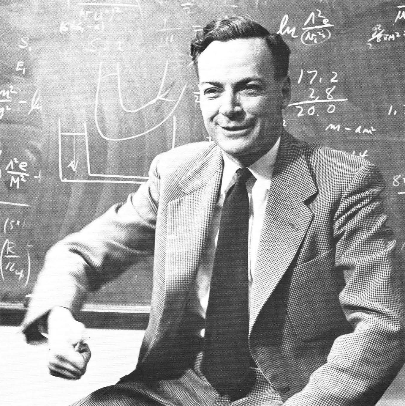
Nature isn’t classical, dammit, and if you want to make a simulation of nature, you’d better make it quantum mechanical.
Richard Feynman
84
In his 1982 paper “Simulating Physics with Computers,” Richard Feynman, 1965 Nobel Laureate in Physics, said he wanted to “talk about the possibility that there is to be an exact simulation, that the computer will do exactly the same as nature.” He then made the statement above, asserting that nature doesn’t especially make itself amenable to computation via classical binary computers.
In this chapter, we begin to explore how quantum computing differs from classical computing. Classical computing drives smartphones, laptops, Internet servers, mainframes, high-performance computers, and even the processors in automobiles.
We examine several use cases where quantum computing may someday help us solve today’s intractable problems using classical methods on classical computers. This is to motivate you to learn about the underpinnings and details of quantum computers I discuss throughout the book.
No single book on this topic can be complete. The technology and potential use cases are moving targets as we innovate and create better hardware and software. My goal here is to prepare you to delve more deeply into the science, coding, and applications of quantum computing.
Topics covered in this chapter
- 1.1. The mysterious quantum bit
- 1.2. I’m awake!
- 1.3. Why quantum computing is different
- 1.5. Applications to financial services
- 1.6. What about cryptography?
- 1.7. Summary
1.1 The mysterious quantum bit
Suppose I am standing in a room with a single overhead light and a switch that turns the light on or off. This is a normal switch, so I can’t dim the light. It is either entirely on or entirely off. I can change it at will, but this is the only thing I can do to the switch. There is a single door to the room and no windows. When the door is closed, I cannot see any light.

I can stay in the room, or I may leave it. The light is always on or off based on the position of the switch.
Now, I’m going to do some rewiring. I’m replacing the switch with one located in another part of the building. I can’t see the light from there, but once again, whether it’s on or off is determined solely by the two positions of the switch.
If I walk to the room with the light and open the door, I can see whether it is lit or dark. I can walk in and out of the room as many times as I want. The status of the light is still determined by that remote switch being on or off. This is a “classical” light.
Let’s imagine a quantum light and switch, which I’ll call a qu-light and qu-switch, respectively.
When I walk into the room with the qu-light, it is always on or off, just like before. The qu-switch is unusual in that it is shaped like a sphere, with the topmost point (the “north pole”) being OFF and the bottommost (the “south pole”) being ON. A line is etched around the middle, as shown in Figure 1.1.

The interesting part happens when I cannot see the qu-light when I am in a different part of the building from the one the qu-switch.
I control the qu-switch by placing my index finger on the qu-switch sphere. If I place my finger on the north pole, the qu-light is off. If I put it on the south, the qu-light is on. You can go into the room and check. You will always get these results.
If I move my finger anywhere else on the qu-switch sphere, the qu-light may be on or off when you check. If you do not check, the qu-light is in an indeterminate state. It is not dimmed, it is not on or off; it just exists with some probability of being on or off when seen. This is unusual!
You remove the indeterminacy when you open the door and see the qu-light. It will be on or off. Moreover, the switch is forced to the north or south pole, corresponding to the state of the qu-light when you see it.
Observing the qu-light forced it into either the on or off state. I don’t have to see the qu-light fixture itself. If I open the door a tiny bit, enough to see if any light is shining, that is enough.
If I place a video camera in the room with the qu-light and watch the light when I put my finger on the qu-switch, the qu-switch behaves like a normal switch. I am prevented from touching the qu-switch anywhere other than the top or bottom, just as a normal switch only has two positions.
If you or I are not observing the qu-light in any way, does it make a difference where I touch the qu-switch? Will touching it in the northern or southern hemisphere influence whether it will be on or off when I observe the qu-light?
Yes. Touching it closer to the north pole or the south pole will make the probability of the qu-light being off or on, respectively, higher. If I put my finger on the circle between the poles, the equator, the probability of the light being on or off will be exactly 50–50.
We call what I just described a two-state quantum system. When no one observes it, the qu-light is in a superposition of being on and off. We explore superposition in section 7.1. superposition two-state quantum system
While this may seem bizarre, evidently, nature works this way. For example, electrons have a property called “spin,” and with this, they are two-state quantum systems. The photons that make up light itself are two-state quantum systems via polarization. We return to this in section 11.9.3 when we look at polarization (as in Polaroid® sunglasses).
More to the point of this book, however, a quantum bit, more commonly known as a qubit, is a two-state quantum system. It extends and complements the classical computing notion of a bit, which can only be 0 or 1. The qubit is the basic information unit in quantum computing. qubit quantum$bit Bloch sphere
This book is about how we manipulate qubits to solve problems that currently appear intractable using just classical computing. It seems that just sticking to 0 or 1 will not be sufficient to solve some problems that would otherwise need impractical amounts of time or memory.
With a qubit, we replace the terminology and notation of on or off, 1 or 0, with the symbols |1⟩ and |0⟩, respectively. Instead of qu-lights, it’s qubits from now on.

In Figure 1.2, we indicate the position of your finger on the qu-switch by two angles, θ (theta) and φ (phi). The picture itself is called a Bloch sphere and is a standard representation of a qubit, as we shall see in section 7.5.
1.2 I’m awake!
What if we could do chemistry inside a computer instead of in a test tube or beaker in the laboratory? What if running a new experiment was as simple as running an app and completing it in a few seconds?
For this to work, we would want it to happen with full fidelity. The atoms and molecules as modeled in the computer should behave exactly like they do in the test tube. The chemical reactions in the physical world would have precise computational analogs. We would need a fully faithful simulation. simulation
If we could do this at scale, we might be able to compute the molecules we want and need. These might be for new materials for shampoos or even alloys for cars and airplanes. Perhaps we could more efficiently discover medicines that we customize for your exact physiology. Maybe we could get better insight into how proteins fold, thereby understanding their function and possibly creating custom enzymes to change our body chemistry positively.
Is this plausible? We have massive supercomputers that can run all kinds of simulations. Can we model molecules in the above ways today?
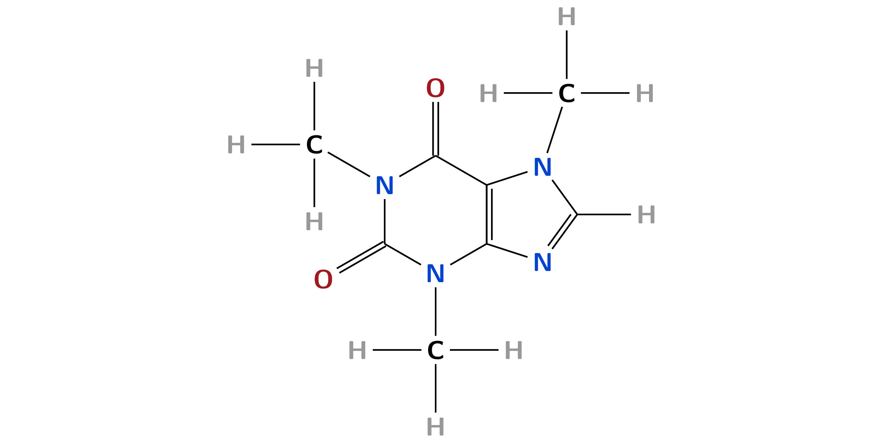
Let’s start with C8H10N4O2 – 1,3,7-Trimethylxanthine. This is a fancy name for a molecule that millions of people worldwide enjoy every day: caffeine. Figure 1.3 shows its structure. caffeine
An 8-ounce cup of coffee contains approximately 95 mg of caffeine, which translates to roughly 2.95 × 10²⁰ molecules. Written out, this is
295,000,000,000,000,000,000 molecules.
A 12-ounce can of a popular cola drink has 32 mg of caffeine, the diet version has 42 mg, and energy drinks often have about 77 mg. 134
Exercise 1.1
How many molecules of caffeine do you consume a day?
These numbers are large because we are counting physical objects in our universe, which we know is very big. Scientists estimate, for example, that there are between 1049 and 1050 atoms in our planet alone. 82
To put these values in context, one thousand = 103, one million = 106, one billion = 109, and so on. A gigabyte of storage is one billion bytes, and a terabyte is 1012 bytes.
Returning to the question I posed at the beginning of this section, can we model caffeine exactly in a computer? We don’t have to model the huge number of caffeine molecules in a cup of coffee, but can we fully represent a single molecule at a single instant?
Caffeine is a small molecule and contains protons, neutrons, and electrons. In particular, if we look at the energy configuration that determines the structure of the molecule and the bonds that hold it all together, the amount of information to describe this is staggering. In particular, the number of bits, the 0s and 1s, needed is approximately 1048:
10,000,000,000,000,000,000,000,000,000,000,000,000,000,000,000,000 .
From what I said above, this is comparable to 1% to 10% of the number of atoms in the Earth.
This is just one molecule! Yet somehow, nature manages to deal quite effectively with all this information. It handles the single caffeine molecule, to all those in your coffee, tea, or soft drink, to every other molecule that makes up you and the world around you.
How does it do this? We don’t know! Of course, there are theories, and they live at the intersection of physics and philosophy. 133 We do not need to understand it thoroughly to try to harness its capabilities.
We have no hope of providing enough traditional storage to hold this much information. Our dream of exact representation appears to be dashed. This is what Richard Feynman (Figure 1.4) meant in his quote at the beginning of this chapter: “Nature isn’t classical.” Feynman, Richard
However, 160 qubits (quantum bits) could hold 2160 ≈ 1.46 × 1048 bits while the qubits are involved in a computation. To be clear, I’m not saying how we would get all the data into those qubits, and I’m also not saying how many more we would need to do something interesting with the information. It does give us hope, however. We look at some ways of encoding data in qubits in section 13.2.
In the classical case, we will never fully represent the caffeine molecule. In the future, with enough very high-quality qubits in a powerful enough quantum computing system, we may be able to perform chemistry in a computer.
To learn more
Quantum chemistry is not an area of science in which you can say a few words and easily make clear how we might eventually use quantum computers to compute molecular properties and protein folding configurations, for example. Nevertheless, the caffeine example above is an example of quantum simulation. chemistry
For an excellent survey of the history and state of the art of quantum computing applied to chemistry as of 2019, see Cao et al. 36 For the specific problem of understanding how to scale quantum simulations of molecules and the crossover from High-Performance Computers (HPC), see Kandala et al. 119
1.3 Why quantum computing is different
I can write a simple app on a classical computer that simulates a coin flip. This app might be for my phone or laptop.
Instead of heads or tails, let’s use 1 and 0. The routine, which I call R, starts with one of those values and randomly returns one or the other. That is, 50% of the time it returns 1, and 50% of the time it returns 0. We have no knowledge whatsoever of how R does what it does. When you see “R,” think “random.”
This routine is a “fair flip.” It is not weighted to prefer one result or the other slightly. Whether we can produce a truly random result on a classical computer is another question. Let’s assume our app is fair.
If I apply R to 1, half the time I expect that same value and the other half 0. The same is true if I apply R to 0. I’ll call these applications R(1) and R(0), respectively.

If I look at the result of R(1) or R(0) in Figure 1.5, there is no way to tell if I started with 1 or 0. This process is like a secret coin flip, where I can’t know whether I began with heads or tails by looking at how the coin has landed. By “secret coin flip,” I mean that someone else does it, and I can see the result, but I have no knowledge of the mechanics of the flip itself or the starting state of the coin.
If R(1) and R(0) are randomly 1 and 0, what happens when I apply R twice?
I write this as R(R(1)) and R(R(0)). It’s the same answer: random result with an equal split. The same thing happens no matter how many times we apply R. The result is random, and we can’t reverse things to learn the initial value. In the language of section 4.1, R is not invertible. function$invertible
Now for the quantum version. Instead of R, I use H, which we learn about in section 7.6. It, too, returns 0 or 1 with equal chance, but it has two interesting properties:
- It is reversible. Though it produces a random 1 or 0, starting from either of them, we can always go back and see the value with which we began.
- It is its own reverse (or inverse) operation. Applying it twice in a row is the same as having done nothing at all.
There is a catch, though. You are not allowed to look at the result of what H does the first time if you want to reverse its effect.

If you apply H to 0 or 1, as shown in Figure 1.6, peek at the result, and apply H again to that, it is the same as if you had used R. If you observe what is going on in the quantum case at the wrong time, you are right back at strictly classical behavior.
To summarize, using the coin language: if you flip a quantum coin and then don’t look at it, flipping it again will yield the heads or tails with which you started. If you do look, you get classical randomness.
Exercise 1.2
Compare this behavior with that of the qu-switch and qu-light in section 1.1.
A second area where quantum is different is in how we can work with simultaneous values. Your phone or laptop uses a byte as the individual memory or storage unit. That’s where we get phrases such as “megabyte,” which means one million bytes of information.
We further break down a byte into eight bits, which we’ve seen before. Each bit can be 0 or 1. Doing the math, each byte can represent 28 = 256 different numbers composed of eight 0s or 1s, but it can only hold one value at a time.
Eight qubits can represent all 256 values at the same time.
This representation is enabled not only through superposition, but also through entanglement, where we can tightly tie together the behavior of two or more qubits. These give us the (literally) exponential growth in the amount of working memory that we saw with a quantum representation of caffeine in section 1.2. We explore entanglement in section 8.2.
1.4 Applications to artificial intelligence
Artificial intelligence (AI) and one of its subsets, machine learning, are broad collections of data-driven techniques and models. They help find patterns in information, learn from the information, and automatically perform tasks more “intelligently.” They also give humans help and insight that might have been difficult to get otherwise. AI machine learning artificial intelligence
Here is a way to start thinking about how quantum computing might apply to large, complicated, computation-intensive systems of processes such as those found in AI and elsewhere. These three cases are, in some sense, the “small, medium, and large” ways quantum computing might complement classical techniques:
- There is a single mathematical computation somewhere in the middle of a software component that might be sped up via a quantum algorithm.
- There is a well-described component of a classical process that could be replaced with a quantum version.
- There is a way to avoid using some classical components entirely in the traditional method because of quantum, or we can replace the entire classical algorithm with a much faster or more effective quantum alternative.
At the time of writing, quantum computers are not “big data” machines. You cannot take millions of information records and provide them as input to a quantum calculation. Instead, quantum may be able to help where the number of inputs is modest, but the computations “blow up” as you start examining relationships or dependencies in the data. Quantum, with its exponentially growing working memory, as we saw in the caffeine example in section 1.2, may be able to control and work with the blow-up. (See section 2.7 for a discussion of exponential growth.)
In the future, however, quantum computers may be able to input, output, and process much more data. Even if it is only theoretical now, it makes sense to ask if there are quantum algorithms that can be useful in AI someday.
Let’s look at some data. I’m a big baseball fan, and baseball has a lot of statistics associated with it. The analysis of this even has its own name: “sabermetrics.” sabermetrics

Suppose I have a table of statistics for a baseball player given by year, as shown in Figure 1.7. We can make this look more mathematical by creating a matrix of the same data:

Given such information, we can manipulate it using machine learning techniques to predict the player’s future performance or even how other similar players may do. These techniques use the matrix operations we discuss in Chapter 5, “Dimensions.”
There are 30 teams in Major League Baseball in the United States. With their training and feeder “minor league” teams, each major league team may have more than 400 players throughout their systems. That would give us over 12,000 players, each with their complete player histories. There are more statistics than I have listed, so we can easily get more than 100,000 values in our matrix.
As another example, in the area of entertainment, it’s hard to estimate how many movies exist, but it is well above 100,000. For each movie, we can list features such as whether it is a comedy, drama, romance, or action film, and who each actor is. We might also know all members of the directorial and production staff, the geographic locations shown in the film, the languages spoken, and so on. There are hundreds of such features and millions of people who have watched the films!
For each person, we can also add features such as whether they like or dislike a type of movie, actor, scene location, or director. Using all this information, which film should I recommend to you on a Saturday night in December, based on what you and people similar to you like?
Think of each feature or each baseball player or film as a dimension. While you may think of two and three dimensions in nature, we might have thousands or millions of dimensions in AI.
Matrices as above for AI can grow to millions of rows and entries. How can we make sense of them to get insights and see patterns? Aside from manipulating that much information, can we even eventually do the math on classical computers quickly and accurately enough?
While scientists initially thought that quantum algorithms might offer exponential improvements to such classical recommender systems, a 2019 algorithm showed a classical method to gain such a large improvement. 213 An example of a process being exponentially faster is doing something in 6 days instead of 106 = 1 million days. That’s approximately 2,740 years. Tang, Ewin
Tang’s work is a fascinating example of the interplay of progress in classical and quantum algorithms. People who develop algorithms for classical computing look to quantum computing and vice versa. Also, any particular solution to a problem may include classical and quantum components.
Nevertheless, many believe that quantum computing will greatly improve some matrix computations. One such example is the HHL algorithm, whose abbreviation comes from the first letters of the last names of its authors, Aram W. Harrow, Avinatan Hassidim, and Seth Lloyd. This algorithm is an example of case number 1 above. 105 63
Algorithms such as these may find use in fields as diverse as economics and computational fluid dynamics. They also place requirements on the structure and density of the data and may use properties such as the condition number, which we discuss in section 5.13.
To learn more
Completing this book will equip you to read the original paper describing the HHL algorithm and more recent surveys about applying quantum computing to linear algebraic problems. 105
An important problem in machine learning is classification. In its simplest form, a binary classifier separates items into one of two categories or buckets. Depending on the definitions of the categories, it may be more or less easy to do the classification.
Examples of binary categories include:
- book you like or book you don’t like
- comedy movie or dramatic movie
- gluten-free or not gluten-free
- fish dish or chicken dish
- UK football team or Spanish football team
- hot sauce or extremely hot sauce
- cotton shirt or permanent press shirt
- open-source or proprietary
- spam email or valid email
- American League baseball team or National League team
The second example of distinguishing between comedies and dramas may not be well designed, since there are movies that are both.
Mathematically, we can imagine taking some data value as input and classifying it as +1 or –1. We take a reasonably large data set and label each value by hand as a +1 or –1. We then learn from this training set how to classify future data.
Machine learning binary classification algorithms include random forest, k-nearest neighbor, decision tree, neural networks, naive Bayes classifiers, and support vector machines. algorithm$support vector machine algorithm$SVM algorithm$classification
In the training phase, we have a list of pre-classified objects (books, movies, proteins, operating systems, baseball teams, etc.). We then use the above algorithms to learn how to put a new object in one bucket or another.
The support vector machine (SVM) is a straightforward approach with a precise mathematical description. In the two-dimensional case, we try to draw a line separating the objects (represented by points in the plot in Figure 1.8) into one category or the other.

The line should maximize the gap between the sets of objects.

The plot in Figure 1.9 is an example of a line separating the dark gray points below from the light gray ones above.
Given a new point, we plot it and determine whether it is above or below the line. That will classify it as dark or or light gray, respectively.
Suppose we know we correctly classified the point with those above the line. We accept that and move on. If we misclassify the point, we add it to the training set and try to compute a new and better line. This may not be possible.

In the plot in Figure 1.10, I added a new light gray point close to 2 on the vertical axis. With this extra point, there is no line we can compute to separate the points.
Had we represented the objects in three dimensions, we would have tried to find a plane that separated the points with a maximum gap. We would need to compute some new amount that the points are above or below the plane. In geometric terms, if we have x and y only, we must somehow compute a z to work in that third dimension.
For a representation using n dimensions, we try to compute an (n – 1)-dimensional separating hyperplane. We look at two and three dimensions in Chapter 4, “Planes and Circles and Spheres, Oh My,” and the general case in Chapter 5, “Dimensions.” hyperplane

In the three-dimensional plot in Figure 1.11, I take the same values from the last two-dimensional version and lay the coordinate plane flat. I then add a vertical dimension. I push the light gray points below the plane and the dark gray ones above. With this construction, the coordinate plane itself separates the values.
While we can’t separate the points in two dimensions, we can in three dimensions. This kind of mapping into a higher dimension is called a kernel trick. While the coordinate plane might not be the ideal separating hyperplane, it gives you an idea of what we are trying to accomplish. The benefit of kernel functions (as part of the similarly named “trick”) is that we can do far fewer explicit geometric computations than you might expect in these higher-dimensional spaces. kernel$trick kernel$function
It’s worth mentioning now that we don’t need to try quantum methods on small problems that we can handle quite well using traditional means. We won’t see any quantum advantage until the problems are big enough to overcome the quantum circuit overhead versus classical circuits. Also, if we come up with a quantum approach that we can simulate efficiently on a classical computer, we don’t need a quantum computer.
A quantum computer with 1 qubit provides us with a two-dimensional working space. Every time we add a qubit, we double the number of dimensions. This is due to the properties of superposition and entanglement that I introduce in Chapter 7, “One Qubit.” For 10 qubits, we get 210 = 1,024 dimensions. Similarly, for 50 qubits, we get 250 = 1,125,899,906,842,624 dimensions.
Remember all those dimensions for the features, baseball players, and films? We want a sufficiently large quantum computer to perform the AI calculations in a quantum feature space. This is the main point: handle the large number of dimensions coming out of the data in a large quantum feature space. feature space quantum$feature space
There is a quantum approach that can generate the separating hyperplane in the quantum feature space. There is another that skips the hyperplane step and produces a highly accurate classifying kernel function. As the ability to entangle more qubits increases, the successful classification rate also improves. 106 This is an active area of research: how can we use entanglement, which does not exist classically, to find new or better patterns than we can with strictly traditional methods?
To learn more
Researchers are writing an increasing number of papers connecting quantum computing with machine learning and other AI techniques, but the results are somewhat fragmented. 236 We return to this topic in Chapter 13, “Introduction to Quantum Machine Learning.” I warn you again that quantum computers cannot process much data now!
For an advanced application of machine learning for quantum computing and chemistry, see Torlai et al. 216 I introduce machine learning and classification methods in Chapter 15 of Dancing with Python. 211
1.5 Applications to financial services
Suppose we have a circle of radius 1 inscribed in a square, as in Figure 1.12. The sides of the square have length 2, and the square’s area is 4 = 2 × 2. What is the area A of the circle?
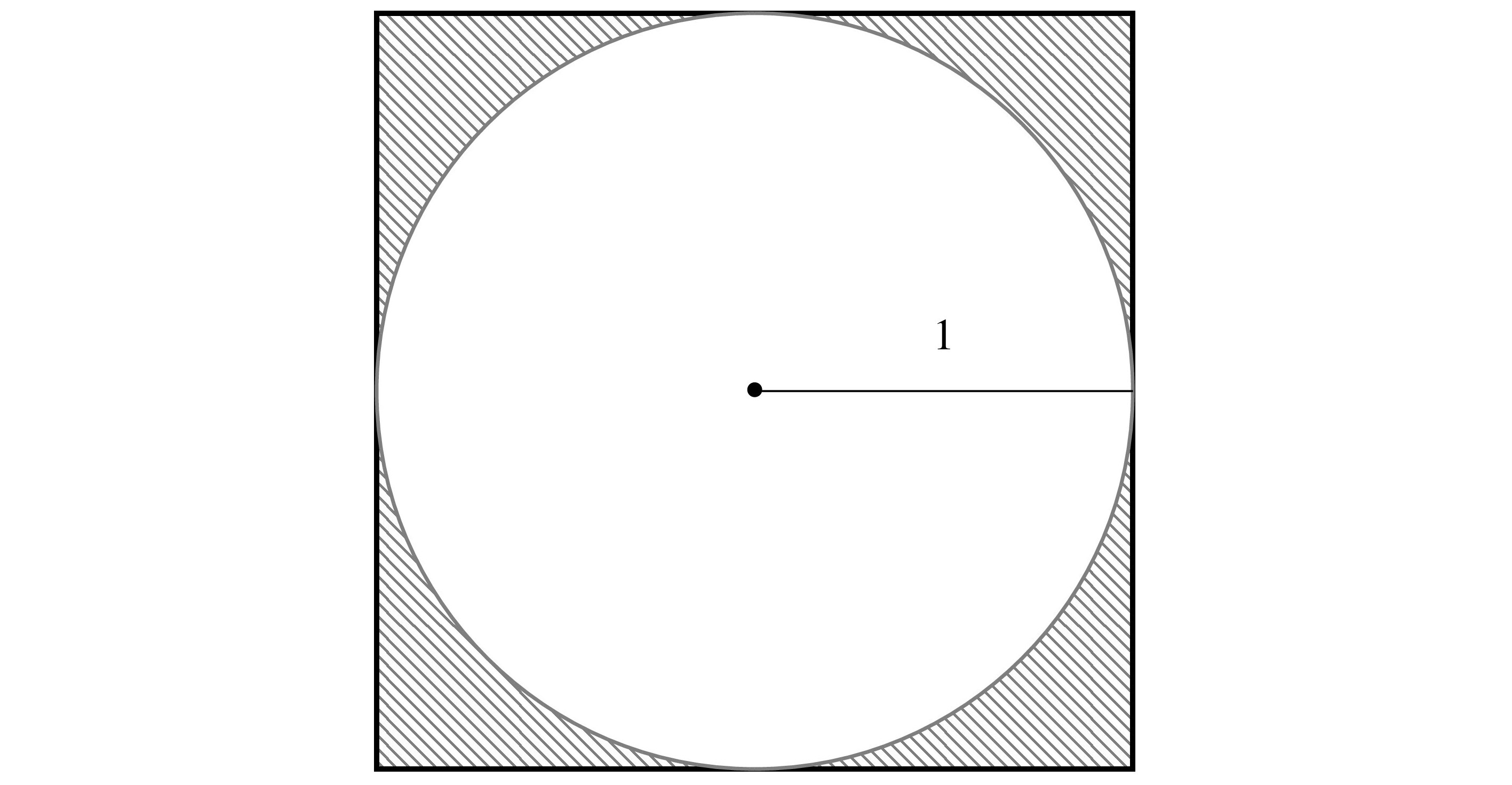
Before you try to remember your geometric area formulas, let’s compute the area of a circle using ratios and some experiments.
Suppose we drop some number N of coins onto the square and count how many have their centers on or inside the circle. If C is this number, then

A ≈ 4C/N.
There is randomness involved here: it’s possible they all land inside the circle or, less likely, outside the circle. For N = 1, we do not get an accurate estimate of A because C/N can only be 0 or 1.
Exercise 1.3
If N = 2, what are the possible estimates of A? What about if N = 3?
We will get a better estimate for A if we choose N large.
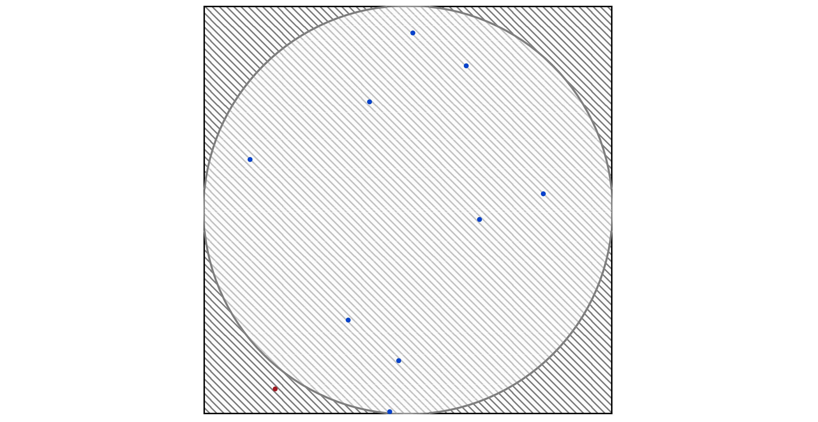
I created 10 points whose centers lie inside the square using Python and its random number generator. The plot in Figure 1.13 shows where they landed. In this case, C = 9, and so A ≈ 3.6.
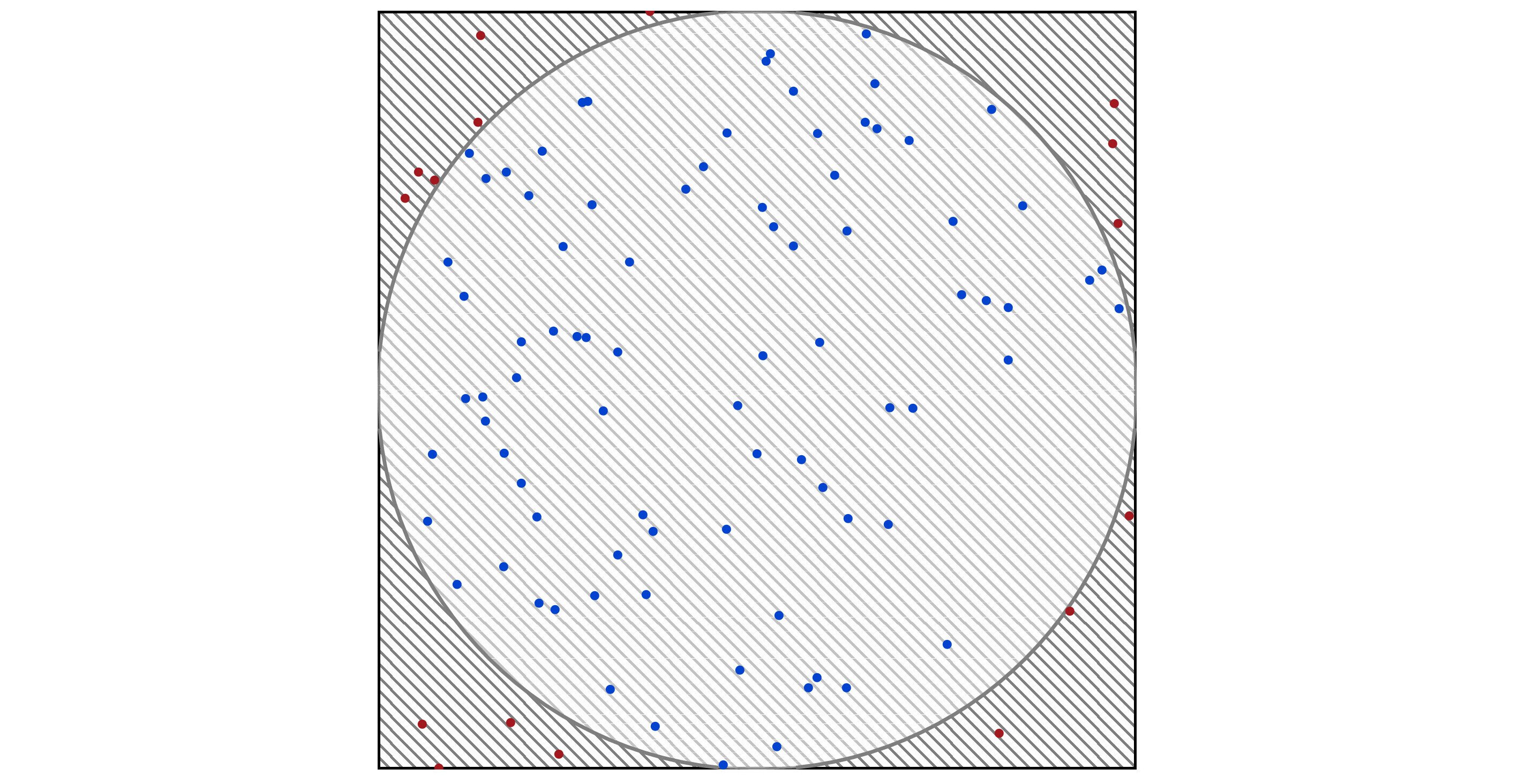
For N = 100, we get a more interesting plot in Figure 1.14 with C = 84 and A ≈ 3.36. Remember, this value would be different if I had generated other random numbers.
The final plot is in Figure 1.15 for N = 500. Now C = 387 and A ≈ 3.096.
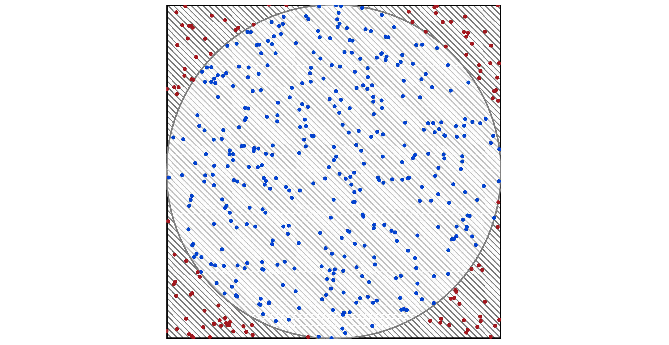
The real value of A is π ≈ 3.1415926. We call this technique Monte Carlo sampling, which goes back to the 1940s. algorithm$Monte Carlo Monte Carlo algorithm
Using the same technique, here are approximations of A for increasingly large N. Remember, we are using random numbers, so these numbers will vary based on the sequence of values used.

That’s a lot of runs, the value of N, to get close to the actual value of π. Nevertheless, this example demonstrates how we can use Monte Carlo sampling techniques to approximate the value of something when we may not have a formula. In this case, we estimated A. For the example, we ignored our knowledge that the formula for the area of a circle is π r2, where r is the circle’s radius.
In section 6.8, we work through the math and show that if we want to estimate π within 0.00001 with a probability of at least 99.9999%, we need N ≥ 82863028. We need to use more than 82 million points! So it is possible to use a Monte Carlo method here, but it is not efficient.
In this example, we know the answer ahead of time by other means. Monte Carlo methods can be a useful tool if we do not know the answer and do not have a nice neat formula to compute. However, the very large number of samples needed to get decent accuracy makes the process computationally intensive. If we can reduce the sample count significantly, we can compute a more accurate result much faster.
Given that the title of this section mentions “finance,” I now note, perhaps unsurprisingly, that quantitative analysts use Monte Carlo methods in computational finance. financial services
The randomness we employ to calculate π translates over into ideas such as uncertainties. Uncertainties can then be related to probabilities, which we use to calculate the risk and rate of return of investments.
Instead of looking at whether a point is inside or outside a circle, for the rate of return, we might consider several factors that go into calculating the risk. For example,
- market size
- share of the market
- selling price
- fixed costs
- operating costs
- obsolescence
- inflation or deflation
- national monetary policy
- weather
- political factors and election results
For each of these or any other factor relevant to the particular investment, we quantify them and assign probabilities to the possible results. In a weighted way, we combine all possible combinations to compute risk. This is a function that we cannot calculate all at once, but we can use Monte Carlo methods to estimate. Techniques similar to, but more complicated than, the circle analysis in section 6.8, give us how many samples we need to use to get a result within the desired accuracy.
In the circle example, reasonable accuracy can require tens of millions of samples. We might need many orders of magnitude greater for an investment risk analysis. So what do we do?
We can and do use High-Performance Computers (HPC). We can consider fewer possibilities for each factor. For example, we might vary the possible selling prices by larger amounts. We can consult better experts and get more accurate probabilities. This could improve the result but not necessarily the computation time. Or, we can take fewer samples and accept less precise results. HPC
Alternatively, we could consider quantum variations and replacements for Monte Carlo methods. In 2015, Ashley Montanaro 152 described a quadratic speedup using quantum computers. How much improvement does this give us? Instead of the 82 million samples required for the circle calculation with the above accuracy, we could do it in something closer to 9,000 samples (9055 ≈ √82000000). Montanaro, Ashley
In 2019, Stamatopoulos et al. showed methods and considerations for pricing financial options using quantum computing systems. 206
I want to stress that to do this, we need much larger, more accurate, and more powerful quantum computers than we have at the time of writing. However, like much of the algorithmic work researchers are doing on industry use cases, I believe we are getting on the right path to solve significant problems significantly faster using quantum computation.
By using Monte Carlo methods, we can vary our assumptions and do scenario analysis. If we can eventually use quantum computers to significantly reduce the number of samples, we can look at far more scenarios much faster.
To learn more
David Hertz’ original 1964 paper in the Harvard Business Review is a very readable introduction to Monte Carlo methods for risk analysis without ever using the phrase “Monte Carlo.” 110 A more recent paper gives more of the history of these methods and applies them to marketing analytics. 87
My goal with this book is to give you enough of an introduction to quantum computing so that you can read industry-specific quantum use cases and research papers. For example, to learn about modern quantum algorithmic approaches to risk analysis, see the articles by Woerner, Egger, et al. 237 76 Some early results on heuristics using quantum computation for transaction settlements are covered in Braine et al. 23
1.6 What about cryptography?
You may have seen media headlines such as
Quantum Security Apocalypse!!!
Y2K??? Get ready for Q2K!!!
Quantum Computing Will Break All Internet Security!!!
These breathless announcements grab your attention and frequently contain egregious errors about quantum computing and security. Let’s look at the root of the concerns and insert some reality into the discussion.
RSA (Rivest-Shamir-Adleman) is a commonly used security protocol, and it works something like this:
- You want to allow others to send you secure communications. This means you give them what they need to encrypt their messages before sending them. You and only you can decrypt what they then give you.
- You publish a public key used to encrypt these messages intended for you. Anyone who has access to the key can use it.
- There is an additional key, your private key. You and only you have it. With it, you can decrypt and read encrypted messages. 190
Though I phrased this in terms of messages sent to you, the scheme is adaptable for sending transaction and purchase data across the Internet and storing information securely in a database.
Indeed, if anyone steals your private key, there is a cybersecurity emergency. Quantum computing has nothing to do with physically taking your private key or convincing you to give it to a bad person.
What if I could compute your private key from the public key?
The public key for RSA looks like a pair of numbers (e, n) where n is a very large integer that is the product of two primes. We’ll call these primes numbers p and q. For example, if p = 982451653 and q = 899809343, then n = p × q = 884019176415193979.
Your private key looks like a pair of integers (d, n) using the very same n as in the public key. It is the d part you must keep secret.
Here’s the potential problem: if someone can quickly factor n into p and q, then they can compute d. That is, fast integer factorization leads to breaking RSA encryption. 204
Though multiplication is very easy and can be done using the method you learned early in your education, factoring can be very, very hard. For products of certain pairs of primes, factorization using known classical methods could take hundreds or thousands of years.
Given this, unless d is stolen or given away, you might feel pretty comfortable about security. But what if there is another way of factoring involving nonclassical computers?
In 1995, Peter Shor published a quantum algorithm for integer factorization that is almost exponentially faster than known classical methods. We analyze Shor’s factoring algorithm in section 10.7. Shor, Peter
This sounds like a major problem! Here is where many articles about quantum computing and security start to go crazy. The key question is, how powerful and of what quality must a quantum computing system be to perform this factorization?
At the time of writing, scientists and engineers are building quantum computers with low four-digit numbers of physical qubits. For example, IBM researchers have a demonstrated qubit count of 1,121. 37 A physical qubit is the hardware implementation of the logical qubits we start discussing in Chapter 7, “One Qubit.”
Physical qubits have noise that causes errors in computation. Shor’s factoring algorithm requires fully fault-tolerant, error-corrected qubits. We can detect and correct errors that occur in logical qubits. This happens today in the memory and data storage in your laptop and smartphone. We explore quantum error correction in section 11.5. logical qubit qubit$logical
As a rule of thumb, assume it will take 1,000 very good physical qubits to make one logical qubit. This estimate varies by the researcher, the degree of marketing hype, and wishful thinking, but I believe 1,000 is reasonable. We discuss the relationship between the two kinds of qubits in Chapter 11, “Getting Physical.” Meanwhile, we are in the Noisy Intermediate-Scale Quantum, or NISQ, era. Physicist John Preskill coined the term NISQ in 2018. Although Preskill initially thought these systems would have between 50 and 100 qubits, or at most a few hundred, it seems apparent that the power of NISQ machines may still be limited even if they have several thousand physical qubits. 172 Preskill, John NISQ Noisy Intermediate-Scale Quantum era

A further estimate is that it will take 2 × 107 = 20 million physical qubits to use Shor’s algorithm to factor the values of n used in RSA today. That’s approximately twenty thousand logical qubits. On the one hand, we have quantum computers with two or three digits worth of physical qubits. We’ll need seven digits’ worth for Shor’s factoring algorithm to break RSA. That’s a huge difference. 91
These numbers may be too conservative, but I don’t think by much. If anyone quotes you much smaller numbers, try to understand their motivation and what data they are using.
There’s a good chance we won’t get quantum computers this powerful until 2035 or much later. We may never get such powerful machines. Assuming we will, what should you do now?
First, you should move to so-called “post-quantum” or “quantum-proof” encryption protocols. These are being standardized at NIST, the National Institute of Standards and Technology, in the United States by an international team of researchers. We believe these protocols can’t be broken by quantum computing systems, as RSA and some of the other classical protocols might be eventually.
You may think you have plenty of time to change over your transactional systems. How long will it take to do that? Financial institutions can take ten years or more to implement new security technology.
Of greater immediate importance is your data. Will it be a problem if someone can crack your database security in 15, 30, or 50 years? For most organizations, the answer is a loud YES. Start looking at hardware and software encryption support for your data using the new post-quantum security standards.
Finally, quantum or no quantum, if you do not have good cybersecurity and encryption strategies and implementations in place now, you are exposed. Fix them. Listen to the people who make quantum computing systems to get a good idea of when hackers might use quantum algorithms to break encryption schemes. All others deal with second and third-hand knowledge.
To learn more
Estimates for when and if quantum computing may pose a cybersecurity threat vary significantly. Any study on the topic must be updated as technology evolves. The most complete analysis at the time of writing this book appears to be Mosca and Piani. 156
1.7 Summary
In this first chapter, we examined what motivates the recent interest in quantum computers. The lone 1s and 0s of classical computing bits are extended and complemented by the infinite states of qubits, also known as quantum bits. The properties of superposition and entanglement give us access to many dimensions of working memory that are unavailable to classical computers.
Industry use cases for quantum computing are nascent, but the areas where experts believe it will be applicable sooner are chemistry, materials science, and financial services. AI is another area where quantum may boost performance for some calculations.
There has been confusion in traditional and social media about the interplay of security, information encryption, and quantum computing. The major areas of misunderstanding are the necessary performance requirements and the timeline.
In the next chapter, we look at classical bit-based computing to more precisely and technically explore how quantum computing may help us attack problems that are otherwise impossible today. In Chapter 3, “More Numbers Than You Can Imagine,” through Chapter 6, “What Do You Mean “Probably”?,” we work through the mathematics necessary for you to see how quantum computing works. There is a lot to cover, but it is worth it to be able to go deeper than a merely superficial understanding of the “whats,” “hows,” and “whys” of quantum computing.