


 Download code from GitHub
Machine learning teaches machines to learn to carry out tasks by themselves. It is that simple. The complexity comes with the details, and that is most likely the reason you are reading this book.
Maybe you have too much data and too little insight. You hope that using machine learning algorithms you can solve this challenge, so you started digging into the algorithms. But after some time you were puzzled: Which of the myriad of algorithms should you actually choose?
Alternatively, maybe you are in general interested in machine learning and for some time you have been reading blogs and articles about it. Everything seemed to be magic and cool, so you started your exploration and fed some toy data into a decision tree or a support vector machine. However, after you successfully applied it to some other data, you wondered: Was the whole setting right? Did you get the optimal results? And how do you know whether there are no better algorithms? Or whether your data was the right one?
Welcome to the club! Both of us (authors) were at those stages looking for information that tells the stories behind the theoretical textbooks about machine learning. It turned out that much of that information was "black art" not usually taught in standard text books. So in a sense, we wrote this book to our younger selves. A book that not only gives a quick introduction into machine learning, but also teaches lessons we learned along the way. We hope that it will also give you a smoother entry to one of the most exciting fields in Computer Science.
The goal of machine learning is to teach machines (software) to carry out tasks by providing them a couple of examples (how to do or not do the task). Let's assume that each morning when you turn on your computer, you do the same task of moving e-mails around so that only e-mails belonging to the same topic end up in the same folder. After some time, you might feel bored and think of automating this chore. One way would be to start analyzing your brain and write down all rules your brain processes while you are shuffling your e-mails. However, this will be quite cumbersome and always imperfect. While you will miss some rules, you will over-specify others. A better and more future-proof way would be to automate this process by choosing a set of e-mail meta info and body/folder name pairs and let an algorithm come up with the best rule set. The pairs would be your training data, and the resulting rule set (also called model) could then be applied to future e-mails that we have not yet seen. This is machine learning in its simplest form.
Of course, machine learning (often also referred to as Data Mining or Predictive Analysis) is not a brand new field in itself. Quite the contrary, its success over the recent years can be attributed to the pragmatic way of using rock-solid techniques and insights from other successful fields like statistics. There the purpose is for us humans to get insights into the data, for example, by learning more about the underlying patterns and relationships. As you read more and more about successful applications of machine learning (you have checked out www.kaggle.com already, haven't you?), you will see that applied statistics is a common field among machine learning experts.
As you will see later, the process of coming up with a decent ML approach is never a waterfall-like process. Instead, you will see yourself going back and forth in your analysis, trying out different versions of your input data on diverse sets of ML algorithms. It is this explorative nature that lends itself perfectly to Python. Being an interpreted high-level programming language, it seems that Python has been designed exactly for this process of trying out different things. What is more, it does this even fast. Sure, it is slower than C or similar statically typed programming languages. Nevertheless, with the myriad of easy-to-use libraries that are often written in C, you don't have to sacrifice speed for agility.
This book will give you a broad overview of what types of learning algorithms are currently most used in the diverse fields of machine learning, and where to watch out when applying them. From our own experience, however, we know that doing the "cool" stuff, that is, using and tweaking machine learning algorithms such as support vector machines, nearest neighbor search, or ensembles thereof, will only consume a tiny fraction of the overall time of a good machine learning expert. Looking at the following typical workflow, we see that most of the time will be spent in rather mundane tasks:
Reading in the data and cleaning it
Exploring and understanding the input data
Analyzing how best to present the data to the learning algorithm
Choosing the right model and learning algorithm
Measuring the performance correctly
When talking about exploring and understanding the input data, we will need a bit of statistics and basic math. However, while doing that, you will see that those topics that seemed to be so dry in your math class can actually be really exciting when you use them to look at interesting data.
The journey starts when you read in the data. When you have to answer questions such as how to handle invalid or missing values, you will see that this is more an art than a precise science. And a very rewarding one, as doing this part right will open your data to more machine learning algorithms and thus increase the likelihood of success.
With the data being ready in your program's data structures, you will want to get a real feeling of what animal you are working with. Do you have enough data to answer your questions? If not, you might want to think about additional ways to get more of it. Do you even have too much data? Then you probably want to think about how best to extract a sample of it.
Often you will not feed the data directly into your machine learning algorithm. Instead you will find that you can refine parts of the data before training. Many times the machine learning algorithm will reward you with increased performance. You will even find that a simple algorithm with refined data generally outperforms a very sophisticated algorithm with raw data. This part of the machine learning workflow is called feature engineering, and is most of the time a very exciting and rewarding challenge. You will immediately see the results of being creative and intelligent.
Choosing the right learning algorithm, then, is not simply a shootout of the three or four that are in your toolbox (there will be more you will see). It is more a thoughtful process of weighing different performance and functional requirements. Do you need a fast result and are willing to sacrifice quality? Or would you rather spend more time to get the best possible result? Do you have a clear idea of the future data or should you be a bit more conservative on that side?
Finally, measuring the performance is the part where most mistakes are waiting for the aspiring machine learner. There are easy ones, such as testing your approach with the same data on which you have trained. But there are more difficult ones, when you have imbalanced training data. Again, data is the part that determines whether your undertaking will fail or succeed.
We see that only the fourth point is dealing with the fancy algorithms. Nevertheless, we hope that this book will convince you that the other four tasks are not simply chores, but can be equally exciting. Our hope is that by the end of the book, you will have truly fallen in love with data instead of learning algorithms.
To that end, we will not overwhelm you with the theoretical aspects of the diverse ML algorithms, as there are already excellent books in that area (you will find pointers in the Appendix). Instead, we will try to provide an intuition of the underlying approaches in the individual chapters—just enough for you to get the idea and be able to undertake your first steps. Hence, this book is by no means the definitive guide to machine learning. It is more of a starter kit. We hope that it ignites your curiosity enough to keep you eager in trying to learn more and more about this interesting field.
In the rest of this chapter, we will set up and get to know the basic Python libraries NumPy and SciPy and then train our first machine learning using scikit-learn. During that endeavor, we will introduce basic ML concepts that will be used throughout the book. The rest of the chapters will then go into more detail through the five steps described earlier, highlighting different aspects of machine learning in Python using diverse application scenarios.
We try to convey every idea necessary to reproduce the steps throughout this book. Nevertheless, there will be situations where you are stuck. The reasons might range from simple typos over odd combinations of package versions to problems in understanding.
In this situation, there are many different ways to get help. Most likely, your problem will already be raised and solved in the following excellent Q&A sites:
http://metaoptimize.com/qa: This Q&A site is laser-focused on machine learning topics. For almost every question, it contains above average answers from machine learning experts. Even if you don't have any questions, it is a good habit to check it out every now and then and read through some of the answers.
http://stats.stackexchange.com: This Q&A site is named Cross Validated, similar to MetaOptimize, but is focused more on statistical problems.
http://stackoverflow.com: This Q&A site is much like the previous ones, but with broader focus on general programming topics. It contains, for example, more questions on some of the packages that we will use in this book, such as SciPy or matplotlib.
#machinelearning on https://freenode.net/: This is the IRC channel focused on machine learning topics. It is a small but very active and helpful community of machine learning experts.
http://www.TwoToReal.com: This is the instant Q&A site written by the authors to support you in topics that don't fit in any of the preceding buckets. If you post your question, one of the authors will get an instant message if he is online and be drawn in a chat with you.
As stated in the beginning, this book tries to help you get started quickly on your machine learning journey. Therefore, we highly encourage you to build up your own list of machine learning related blogs and check them out regularly. This is the best way to get to know what works and what doesn't.
The only blog we want to highlight right here (more in the Appendix) is http://blog.kaggle.com, the blog of the Kaggle company, which is carrying out machine learning competitions. Typically, they encourage the winners of the competitions to write down how they approached the competition, what strategies did not work, and how they arrived at the winning strategy. Even if you don't read anything else, this is a must.
Assuming that you have Python already installed (everything at least as recent as 2.7 should be fine), we need to install NumPy and SciPy for numerical operations, as well as matplotlib for visualization.
Before we can talk about concrete machine learning algorithms, we have to talk about how best to store the data we will chew through. This is important as the most advanced learning algorithm will not be of any help to us if it will never finish. This may be simply because accessing the data is too slow. Or maybe its representation forces the operating system to swap all day. Add to this that Python is an interpreted language (a highly optimized one, though) that is slow for many numerically heavy algorithms compared to C or FORTRAN. So we might ask why on earth so many scientists and companies are betting their fortune on Python even in highly computation-intensive areas?
The answer is that, in Python, it is very easy to off-load number crunching tasks to the lower layer in the form of C or FORTRAN extensions. And that is exactly what NumPy and SciPy do (http://scipy.org/Download). In this tandem, NumPy provides the support of highly optimized multidimensional arrays, which are the basic data structure of most state-of-the-art algorithms. SciPy uses those arrays to provide a set of fast numerical recipes. Finally, matplotlib (http://matplotlib.org/) is probably the most convenient and feature-rich library to plot high-quality graphs using Python.
Luckily, for all major operating systems, that is, Windows, Mac, and Linux, there are targeted installers for NumPy, SciPy, and matplotlib. If you are unsure about the installation process, you might want to install Anaconda Python distribution (which you can access at https://store.continuum.io/cshop/anaconda/), which is driven by Travis Oliphant, a founding contributor of SciPy. What sets Anaconda apart from other distributions such as Enthought Canopy (which you can download from https://www.enthought.com/downloads/) or Python(x,y) (accessible at http://code.google.com/p/pythonxy/wiki/Downloads), is that Anaconda is already fully Python 3 compatible—the Python version we will be using throughout the book.
Let's walk quickly through some basic NumPy examples and then take a look at what SciPy provides on top of it. On the way, we will get our feet wet with plotting using the marvelous Matplotlib package.
For an in-depth explanation, you might want to take a look at some of the more interesting examples of what NumPy has to offer at http://www.scipy.org/Tentative_NumPy_Tutorial.
You will also find the NumPy Beginner's Guide - Second Edition, Ivan Idris, by Packt Publishing, to be very valuable. Additional tutorial style guides can be found at http://scipy-lectures.github.com, and the official SciPy tutorial at http://docs.scipy.org/doc/scipy/reference/tutorial.
So let's import NumPy and play a bit with it. For that, we need to start the Python interactive shell:
>>> import numpy
>>> numpy.version.full_version
1.8.1
As we do not want to pollute our namespace, we certainly should not use the following code:
>>> from numpy import *
Because, for instance, numpy.array will potentially shadow the array package that is included in standard Python. Instead, we will use the following convenient shortcut:
>>> import numpy as np
>>> a = np.array([0,1,2,3,4,5])
>>> a
array([0, 1, 2, 3, 4, 5])
>>> a.ndim
1
>>> a.shape
(6,)
So, we just created an array like we would create a list in Python. However, the NumPy arrays have additional information about the shape. In this case, it is a one-dimensional array of six elements. No surprise so far.
We can now transform this array to a two-dimensional matrix:
>>> b = a.reshape((3,2))
>>> b
array([[0, 1],
       [2, 3],
       [4, 5]])
>>> b.ndim
2
>>> b.shape
(3, 2)
The funny thing starts when we realize just how much the NumPy package is optimized. For example, doing this avoids copies wherever possible:
>>> b[1][0] = 77
>>> b
array([[ 0,  1],
       [77,  3],
       [ 4,  5]])
>>> a
array([ 0,  1, 77,  3,  4,  5])
In this case, we have modified value 2 to 77 in b, and immediately see the same change reflected in a as well. Keep in mind that whenever you need a true copy, you can always perform:
>>> c = a.reshape((3,2)).copy()
>>> c
array([[ 0,  1],
       [77,  3],
       [ 4,  5]])
>>> c[0][0] = -99
>>> a
array([ 0,  1, 77,  3,  4,  5])
>>> c
array([[-99,   1],
       [ 77,   3],
       [  4,   5]])
Note that here, c and a are totally independent copies.
Another big advantage of NumPy arrays is that the operations are propagated to the individual elements. For example, multiplying a NumPy array will result in an array of the same size with all of its elements being multiplied:
>>> d = np.array([1,2,3,4,5])
>>> d*2
array([ 2,  4,  6,  8, 10])
Similarly, for other operations:
>>> d**2
array([ 1,  4,  9, 16, 25])
Contrast that to ordinary Python lists:
>>> [1,2,3,4,5]*2
[1, 2, 3, 4, 5, 1, 2, 3, 4, 5]
>>> [1,2,3,4,5]**2
Traceback (most recent call last):
  File "<stdin>", line 1, in <module>
TypeError: unsupported operand type(s) for ** or pow(): 'list' and 'int'
Of course by using NumPy arrays, we sacrifice the agility Python lists offer. Simple operations such as adding or removing are a bit complex for NumPy arrays. Luckily, we have both at our hands and we will use the right one for the task at hand.
Part of the power of NumPy comes from the versatile ways in which its arrays can be accessed.
In addition to normal list indexing, it allows you to use arrays themselves as indices by performing:
>>> a[np.array([2,3,4])]
array([77,  3,  4])
Together with the fact that conditions are also propagated to individual elements, we gain a very convenient way to access our data:
>>> a>4
array([False, False,  True, False, False,  True], dtype=bool)
>>> a[a>4]
array([77,  5])
By performing the following command, this can be used to trim outliers:
>>> a[a>4] = 4
>>> a
array([0, 1, 4, 3, 4, 4])
As this is a frequent use case, there is the special clip function for it, clipping the values at both ends of an interval with one function call:
>>> a.clip(0,4)
array([0, 1, 4, 3, 4, 4])
The power of NumPy's indexing capabilities comes in handy when preprocessing data that we have just read in from a text file. Most likely, that will contain invalid values that we will mark as not being a real number using numpy.NAN:
>>> c = np.array([1, 2, np.NAN, 3, 4]) # let's pretend we have read this from a text file
>>> c
array([  1.,   2.,  nan,   3.,   4.])
>>> np.isnan(c)
array([False, False,  True, False, False], dtype=bool)
>>> c[~np.isnan(c)]
array([ 1.,  2.,  3.,  4.])
>>> np.mean(c[~np.isnan(c)])
2.5
Let's compare the runtime behavior of NumPy compared with normal Python lists. In the following code, we will calculate the sum of all squared numbers from 1 to 1000 and see how much time it will take. We perform it 10,000 times and report the total time so that our measurement is accurate enough.
import timeit
normal_py_sec = timeit.timeit('sum(x*x for x in range(1000))',
                              number=10000)
naive_np_sec = timeit.timeit(
                'sum(na*na)',
                setup="import numpy as np; na=np.arange(1000)",
                number=10000)
good_np_sec = timeit.timeit(
                'na.dot(na)',
                setup="import numpy as np; na=np.arange(1000)",
                number=10000)

print("Normal Python: %f sec" % normal_py_sec)
print("Naive NumPy: %f sec" % naive_np_sec)
print("Good NumPy: %f sec" % good_np_sec)

Normal Python: 1.050749 sec
Naive NumPy: 3.962259 sec
Good NumPy: 0.040481 sec
We make two interesting observations. Firstly, by just using NumPy as data storage (Naive NumPy) takes 3.5 times longer, which is surprising since we believe it must be much faster as it is written as a C extension. One reason for this is that the access of individual elements from Python itself is rather costly. Only when we are able to apply algorithms inside the optimized extension code is when we get speed improvements. The other observation is quite a tremendous one: using the dot() function of NumPy, which does exactly the same, allows us to be more than 25 times faster. In summary, in every algorithm we are about to implement, we should always look how we can move loops over individual elements from Python to some of the highly optimized NumPy or SciPy extension functions.
However, the speed comes at a price. Using NumPy arrays, we no longer have the incredible flexibility of Python lists, which can hold basically anything. NumPy arrays always have only one data type.
>>> a = np.array([1,2,3])
>>> a.dtype
dtype('int64')
If we try to use elements of different types, such as the ones shown in the following code, NumPy will do its best to coerce them to be the most reasonable common data type:
>>> np.array([1, "stringy"])
array(['1', 'stringy'], dtype='<U7')
>>> np.array([1, "stringy", set([1,2,3])])
array([1, stringy, {1, 2, 3}], dtype=object)
On top of the efficient data structures of NumPy, SciPy offers a magnitude of algorithms working on those arrays. Whatever numerical heavy algorithm you take from current books on numerical recipes, most likely you will find support for them in SciPy in one way or the other. Whether it is matrix manipulation, linear algebra, optimization, clustering, spatial operations, or even fast Fourier transformation, the toolbox is readily filled. Therefore, it is a good habit to always inspect the scipy module before you start implementing a numerical algorithm.
For convenience, the complete namespace of NumPy is also accessible via SciPy. So, from now on, we will use NumPy's machinery via the SciPy namespace. You can check this easily comparing the function references of any base function, such as:
>>> import scipy, numpy
>>> scipy.version.full_version
0.14.0
>>> scipy.dot is numpy.dot
True
The diverse algorithms are grouped into the following toolboxes:
The toolboxes most interesting to our endeavor are scipy.stats, scipy.interpolate, scipy.cluster, and scipy.signal. For the sake of brevity, we will briefly explore some features of the stats package and leave the others to be explained when they show up in the individual chapters.
Let's get our hands dirty and take a look at our hypothetical web start-up, MLaaS, which sells the service of providing machine learning algorithms via HTTP. With increasing success of our company, the demand for better infrastructure increases to serve all incoming web requests successfully. We don't want to allocate too many resources as that would be too costly. On the other side, we will lose money, if we have not reserved enough resources to serve all incoming requests. Now, the question is, when will we hit the limit of our current infrastructure, which we estimated to be at 100,000 requests per hour. We would like to know in advance when we have to request additional servers in the cloud to serve all the incoming requests successfully without paying for unused ones.
We have collected the web stats for the last month and aggregated them in ch01/data/web_traffic.tsv (.tsv because it contains tab-separated values). They are stored as the number of hits per hour. Each line contains the hour consecutively and the number of web hits in that hour.
The first few lines look like the following:
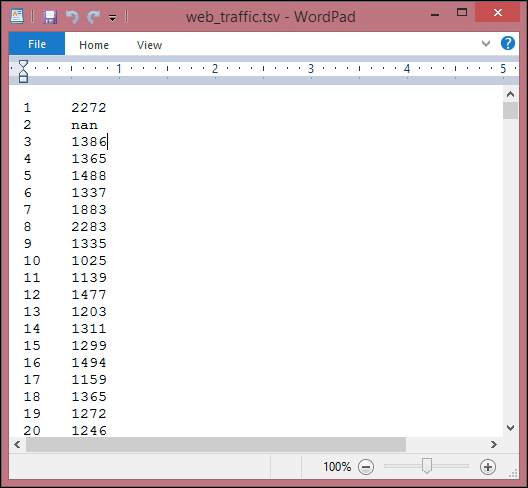
Using SciPy's genfromtxt(), we can easily read in the data using the following code:
>>> import scipy as sp
>>> data = sp.genfromtxt("web_traffic.tsv", delimiter="\t")
We have to specify tab as the delimiter so that the columns are correctly determined.
A quick check shows that we have correctly read in the data:
>>> print(data[:10])
[[  1.00000000e+00   2.27200000e+03]
 [  2.00000000e+00              nan]
 [  3.00000000e+00   1.38600000e+03]
 [  4.00000000e+00   1.36500000e+03]
 [  5.00000000e+00   1.48800000e+03]
 [  6.00000000e+00   1.33700000e+03]
 [  7.00000000e+00   1.88300000e+03]
 [  8.00000000e+00   2.28300000e+03]
 [  9.00000000e+00   1.33500000e+03]
 [  1.00000000e+01   1.02500000e+03]]
>>> print(data.shape)
(743, 2)
As you can see, we have 743 data points with two dimensions.
It is more convenient for SciPy to separate the dimensions into two vectors, each of size 743. The first vector, x, will contain the hours, and the other, y, will contain the Web hits in that particular hour. This splitting is done using the special index notation of SciPy, by which we can choose the columns individually:
x = data[:,0]
y = data[:,1]
There are many more ways in which data can be selected from a SciPy array. Check out http://www.scipy.org/Tentative_NumPy_Tutorial for more details on indexing, slicing, and iterating.
One caveat is still that we have some values in y that contain invalid values, nan. The question is what we can do with them. Let's check how many hours contain invalid data, by running the following code:
>>> sp.sum(sp.isnan(y))
8
As you can see, we are missing only 8 out of 743 entries, so we can afford to remove them. Remember that we can index a SciPy array with another array. Sp.isnan(y) returns an array of Booleans indicating whether an entry is a number or not. Using ~, we logically negate that array so that we choose only those elements from x and y where y contains valid numbers:
>>> x = x[~sp.isnan(y)]
>>> y = y[~sp.isnan(y)]
To get the first impression of our data, let's plot the data in a scatter plot using matplotlib. matplotlib contains the pyplot package, which tries to mimic MATLAB's interface, which is a very convenient and easy to use one as you can see in the following code:
>>> import matplotlib.pyplot as plt
>>> # plot the (x,y) points with dots of size 10
>>> plt.scatter(x, y, s=10)
>>> plt.title("Web traffic over the last month")
>>> plt.xlabel("Time")
>>> plt.ylabel("Hits/hour")
>>> plt.xticks([w*7*24 for w in range(10)],
               ['week %i' % w for w in range(10)])
>>> plt.autoscale(tight=True)
>>> # draw a slightly opaque, dashed grid
>>> plt.grid(True, linestyle='-', color='0.75')
>>> plt.show()
Note
You can find more tutorials on plotting at http://matplotlib.org/users/pyplot_tutorial.html.
In the resulting chart, we can see that while in the first weeks the traffic stayed more or less the same, the last week shows a steep increase:

Now that we have a first impression of the data, we return to the initial question: How long will our server handle the incoming web traffic? To answer this we have to do the following:
Find the real model behind the noisy data points.
Following this, use the model to extrapolate into the future to find the point in time where our infrastructure has to be extended.
When we talk about models, you can think of them as simplified theoretical approximations of complex reality. As such there is always some inferiority involved, also called the approximation error. This error will guide us in choosing the right model among the myriad of choices we have. And this error will be calculated as the squared distance of the model's prediction to the real data; for example, for a learned model function f, the error is calculated as follows:
def error(f, x, y):
    return sp.sum((f(x)-y)**2)
The vectors x and y contain the web stats data that we have extracted earlier. It is the beauty of SciPy's vectorized functions that we exploit here with f(x). The trained model is assumed to take a vector and return the results again as a vector of the same size so that we can use it to calculate the difference to y.
Let's assume for a second that the underlying model is a straight line. Then the challenge is how to best put that line into the chart so that it results in the smallest approximation error. SciPy's polyfit() function does exactly that. Given data x and y and the desired order of the polynomial (a straight line has order 1), it finds the model function that minimizes the error function defined earlier:
fp1, residuals, rank, sv, rcond = sp.polyfit(x, y, 1, full=True)
The polyfit() function returns the parameters of the fitted model function, fp1. And by setting full=True, we also get additional background information on the fitting process. Of this, only residuals are of interest, which is exactly the error of the approximation:
>>> print("Model parameters: %s" % fp1)
Model parameters: [   2.59619213  989.02487106]
>>> print(residuals)
[  3.17389767e+08]
This means the best straight line fit is the following function
f(x) = 2.59619213 * x + 989.02487106.
We then use poly1d() to create a model function from the model parameters:
>>> f1 = sp.poly1d(fp1)
>>> print(error(f1, x, y))
317389767.34
We have used full=True to retrieve more details on the fitting process. Normally, we would not need it, in which case only the model parameters would be returned.
We can now use f1() to plot our first trained model. In addition to the preceding plotting instructions, we simply add the following code:
fx = sp.linspace(0,x[-1], 1000) # generate X-values for plotting
plt.plot(fx, f1(fx), linewidth=4)
plt.legend(["d=%i" % f1.order], loc="upper left")
This will produce the following plot:

It seems like the first 4 weeks are not that far off, although we clearly see that there is something wrong with our initial assumption that the underlying model is a straight line. And then, how good or how bad actually is the error of 317,389,767.34?
The absolute value of the error is seldom of use in isolation. However, when comparing two competing models, we can use their errors to judge which one of them is better. Although our first model clearly is not the one we would use, it serves a very important purpose in the workflow. We will use it as our baseline until we find a better one. Whatever model we come up with in the future, we will compare it against the current baseline.
Let's now fit a more complex model, a polynomial of degree 2, to see whether it better understands our data:
>>> f2p = sp.polyfit(x, y, 2)
>>> print(f2p)
array([  1.05322215e-02,  -5.26545650e+00,   1.97476082e+03])
>>> f2 = sp.poly1d(f2p)
>>> print(error(f2, x, y))
179983507.878
You will get the following plot:

The error is 179,983,507.878, which is almost half the error of the straight line model. This is good but unfortunately this comes with a price: We now have a more complex function, meaning that we have one parameter more to tune inside polyfit(). The fitted polynomial is as follows:
f(x) = 0.0105322215 * x**2 - 5.26545650 * x + 1974.76082
So, if more complexity gives better results, why not increase the complexity even more? Let's try it for degrees 3, 10, and 100.

Interestingly, we do not see d=53 for the polynomial that had been fitted with 100 degrees. Instead, we see lots of warnings on the console:
RankWarning: Polyfit may be poorly conditioned
This means because of numerical errors, polyfit cannot determine a good fit with 100 degrees. Instead, it figured that 53 must be good enough.
It seems like the curves capture and better the fitted data the more complex they get. And also, the errors seem to tell the same story:
Error d=1: 317,389,767.339778
Error d=2: 179,983,507.878179
Error d=3: 139,350,144.031725
Error d=10: 121,942,326.363461
Error d=53: 109,318,004.475556
However, taking a closer look at the fitted curves, we start to wonder whether they also capture the true process that generated that data. Framed differently, do our models correctly represent the underlying mass behavior of customers visiting our website? Looking at the polynomial of degree 10 and 53, we see wildly oscillating behavior. It seems that the models are fitted too much to the data. So much that it is now capturing not only the underlying process but also the noise. This is called overfitting.
At this point, we have the following choices:
Choosing one of the fitted polynomial models.
Switching to another more complex model class. Splines?
Thinking differently about the data and start again.
Out of the five fitted models, the first order model clearly is too simple, and the models of order 10 and 53 are clearly overfitting. Only the second and third order models seem to somehow match the data. However, if we extrapolate them at both borders, we see them going berserk.
Switching to a more complex class seems also not to be the right way to go. What arguments would back which class? At this point, we realize that we probably have not fully understood our data.
So, we step back and take another look at the data. It seems that there is an inflection point between weeks 3 and 4. So let's separate the data and train two lines using week 3.5 as a separation point:
inflection = 3.5*7*24 # calculate the inflection point in hours
xa = x[:inflection] # data before the inflection point
ya = y[:inflection]
xb = x[inflection:] # data after
yb = y[inflection:]

fa = sp.poly1d(sp.polyfit(xa, ya, 1))
fb = sp.poly1d(sp.polyfit(xb, yb, 1))

fa_error = error(fa, xa, ya)
fb_error = error(fb, xb, yb)
print("Error inflection=%f" % (fa_error + fb_error))
Error inflection=132950348.197616
From the first line, we train with the data up to week 3, and in the second line we train with the remaining data.

Clearly, the combination of these two lines seems to be a much better fit to the data than anything we have modeled before. But still, the combined error is higher than the higher order polynomials. Can we trust the error at the end?
Asked differently, why do we trust the straight line fitted only at the last week of our data more than any of the more complex models? It is because we assume that it will capture future data better. If we plot the models into the future, we see how right we are (d=1 is again our initial straight line).

The models of degree 10 and 53 don't seem to expect a bright future of our start-up. They tried so hard to model the given data correctly that they are clearly useless to extrapolate beyond. This is called overfitting. On the other hand, the lower degree models seem not to be capable of capturing the data good enough. This is called underfitting.
So let's play fair to models of degree 2 and above and try out how they behave if we fit them only to the data of the last week. After all, we believe that the last week says more about the future than the data prior to it. The result can be seen in the following psychedelic chart, which further shows how badly the problem of overfitting is.

Still, judging from the errors of the models when trained only on the data from week 3.5 and later, we still should choose the most complex one (note that we also calculate the error only on the time after the inflection point):
Error d=1:   22,143,941.107618
Error d=2:   19,768,846.989176
Error d=3:   19,766,452.361027
Error d=10:  18,949,339.348539
Error d=53:  18,300,702.038119
If we only had some data from the future that we could use to measure our models against, then we should be able to judge our model choice only on the resulting approximation error.
Although we cannot look into the future, we can and should simulate a similar effect by holding out a part of our data. Let's remove, for instance, a certain percentage of the data and train on the remaining one. Then we used the held-out data to calculate the error. As the model has been trained not knowing the held-out data, we should get a more realistic picture of how the model will behave in the future.
The test errors for the models trained only on the time after inflection point now show a completely different picture:
Error d=1: 6397694.386394
Error d=2: 6010775.401243
Error d=3: 6047678.658525
Error d=10: 7037551.009519
Error d=53: 7052400.001761
Have a look at the following plot:

It seems that we finally have a clear winner: The model with degree 2 has the lowest test error, which is the error when measured using data that the model did not see during training. And this gives us hope that we won't get bad surprises when future data arrives.
Finally we have arrived at a model which we think represents the underlying process best; it is now a simple task of finding out when our infrastructure will reach 100,000 requests per hour. We have to calculate when our model function reaches the value 100,000.
Having a polynomial of degree 2, we could simply compute the inverse of the function and calculate its value at 100,000. Of course, we would like to have an approach that is applicable to any model function easily.
This can be done by subtracting 100,000 from the polynomial, which results in another polynomial, and finding its root. SciPy's optimize module has the function fsolve that achieves this, when providing an initial starting position with parameter x0. As every entry in our input data file corresponds to one hour, and we have 743 of them, we set the starting position to some value after that. Let fbt2 be the winning polynomial of degree 2.
>>> fbt2 = sp.poly1d(sp.polyfit(xb[train], yb[train], 2))
>>> print("fbt2(x)= \n%s" % fbt2)
fbt2(x)=
       2
0.086 x - 94.02 x + 2.744e+04
>>> print("fbt2(x)-100,000= \n%s" % (fbt2-100000))
fbt2(x)-100,000=
       2
0.086 x - 94.02 x - 7.256e+04
>>> from scipy.optimize import fsolve
>>> reached_max = fsolve(fbt2-100000, x0=800)/(7*24)
>>> print("100,000 hits/hour expected at week %f" % reached_max[0])
It is expected to have 100,000 hits/hour at week 9.616071, so our model tells us that, given the current user behavior and traction of our start-up, it will take another month until we have reached our capacity threshold.
Of course, there is a certain uncertainty involved with our prediction. To get a real picture of it, one could draw in more sophisticated statistics to find out about the variance we have to expect when looking farther and farther into the future.
And then there are the user and underlying user behavior dynamics that we cannot model accurately. However, at this point, we are fine with the current predictions. After all, we can prepare all time-consuming actions now. If we then monitor our web traffic closely, we will see in time when we have to allocate new resources.
Congratulations! You just learned two important things, of which the most important one is that as a typical machine learning operator, you will spend most of your time in understanding and refining the data—exactly what we just did in our first tiny machine learning example. And we hope that this example helped you to start switching your mental focus from algorithms to data. Then you learned how important it is to have the correct experiment setup and that it is vital to not mix up training and testing.
Admittedly, the use of polynomial fitting is not the coolest thing in the machine learning world. We have chosen it to not distract you by the coolness of some shiny algorithm when we conveyed the two most important messages we just summarized earlier.
So, let's move to the next chapter in which we will dive deep into scikit-learn, the marvelous machine learning toolkit, give an overview of different types of learning, and show you the beauty of feature engineering.

