


 Download code from GitHub
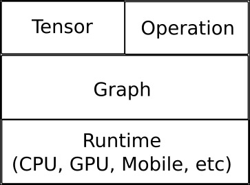
TensorFlow is an open source software library for numerical computation using data flow graphs. Nodes in the graph represent mathematical operations, while the graph edges represent the multidimensional data arrays (tensors) passed between them.
The library includes various functions that enable you to implement and explore the cutting edge Convolutional Neural Network (CNN) and Recurrent Neural Network (RNN) architectures for image and text processing. As the complex computations are arranged in the form of graphs, TensorFlow can be used as a framework that enables you to develop your own models with ease and use them in the field of machine learning.
It is also capable of running in the most heterogeneous environments, from CPUs to mobile processors, including highly-parallel GPU computing, and with the new serving architecture being able to run on very complex mixes of all the named options:
TensorFlow bases its data management on tensors. Tensors are concepts from the field of mathematics, and are developed as a generalization of the linear algebra terms of vectors and matrices.
Talking specifically about TensorFlow, a tensor is just a typed, multidimensional array, with additional operations, modeled in the tensor object.
As previously discussed, TensorFlow uses tensor data structure to represent all data. Any tensor has a static type and dynamic dimensions, so you can change a tensor's internal organization in real-time.
Another property of tensors, is that only objects of the tensor type can be passed between nodes in the computation graph.
Let's now see what the properties of tensors are (from now on, every time we use the word tensor, we'll be referring to TensorFlow's tensor objects).
Tensor ranks represent the dimensional aspect of a tensor, but is not the same as a matrix rank. It represents the quantity of dimensions in which the tensor lives, and is not a precise measure of the extension of the tensor in rows/columns or spatial equivalents.
A rank one tensor is the equivalent of a vector, and a rank one tensor is a matrix. For a rank two tensor you can access any element with the syntax t[i, j]. For a rank three tensor you would need to address an element with t[i, j, k], and so on.
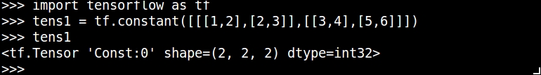
In the following example, we will create a tensor, and access one of its components:
>>> import tensorflow as tf
>>> tens1 = tf.constant([[[1,2],[2,3]],[[3,4],[5,6]]])
>>> print sess.run(tens1)[1,1,0]
5
This is a tensor of rank three, because in each element of the containing matrix, there is a vector element:
|
Rank |
Math entity |
Code definition example |
|
0 |
Scalar |
scalar = 1000 |
|
1 |
Vector |
vector = [2, 8, 3] |
|
2 |
Matrix |
matrix = [[4, 2, 1], [5, 3, 2], [5, 5, 6]] |
|
3 |
3-tensor |
tensor = [[[4], [3], [2]], [[6], [100], [4]], [[5], [1], [4]]] |
|
n |
n-tensor |
... |
The TensorFlow documentation uses three notational conventions to describe tensor dimensionality: rank, shape, and dimension number. The following table shows how these relate to one another:
|
Rank |
Shape |
Dimension number |
Example |
|
0 |
[] |
0 |
4 |
|
1 |
[D0] |
1 |
[2] |
|
2 |
[D0, D1] |
2 |
[6, 2] |
|
3 |
[D0, D1, D2] |
3 |
[7, 3, 2] |
|
n |
[D0, D1, ... Dn-1] |
n-D |
A tensor with shape [D0, D1, ... Dn-1]. |
In the following example, we create a sample rank three tensor, and print the shape of it:
In addition to dimensionality, tensors have a fixed data type. You can assign any one of the following data types to a tensor:
|
Data type |
Python type |
Description |
|---|---|---|
|
|
|
32 bits floating point. |
|
|
|
64 bits floating point. |
|
|
|
8 bits signed integer. |
|
|
|
16 bits signed integer. |
|
|
|
32 bits signed integer. |
|
|
|
64 bits signed integer. |
|
|
|
8 bits unsigned integer. |
|
|
|
Variable length byte arrays. Each element of a tensor is a byte array. |
|
|
|
Boolean. |
We can either create our own tensors, or derivate them from the well-known numpy library. In the following example, we create some numpy arrays, and do some basic math with them:
import tensorflow as tf
import numpy as np
x = tf.constant(np.random.rand(32).astype(np.float32))
y=  tf.constant ([1,2,3])
TensorFlow is interoperable with numpy, and normally the eval() function calls will return a numpy object, ready to be worked with the standard numerical tools.
Tip
We must note that the tensor object is a symbolic handle for the result of an operation, so it doesn't hold the resulting values of the structures it contains. For this reason, we must run the eval() method to get the actual values, which is the equivalent to Session.run(tensor_to_eval).
In this example, we build two numpy arrays, and convert them to tensors:
import tensorflow as tf #we import tensorflow
import numpy as np   #we import numpy
sess = tf.Session() #start a new Session Object
x_data = np.array([[1.,2.,3.],
[3.,2.,6.]]) # 2x3 matrix
x = tf.convert_to_tensor(x_data, dtype=tf.float32) #Finally, we create the tensor, starting from the fload 3x matrix
As with the majority of Python's modules, TensorFlow allows the use of Python's interactive console:
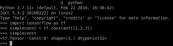
Simple interaction with Python's interpreter and TensorFlow libraries
In the previous figure, we call the Python interpreter (by simply calling Python) and create a tensor of constant type. Then we invoke it again, and the Python interpreter shows the shape and type of the tensor.
We can also use the IPython interpreter, which will allow us to employ a format more compatible with notebook-style tools, such as Jupyter:
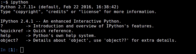
IPython prompt
When talking about running TensorFlow Sessions in an interactive manner, it's better to employ the InteractiveSession object.
Unlike the normal tf.Session class, the tf.InteractiveSession class installs itself as the default session on construction. So when you try to eval a tensor, or run an operation, it will not be necessary to pass a Session object to indicate which session it refers to.
TensorFlow's data flow graph is a symbolic representation of how the computation of the models will work:
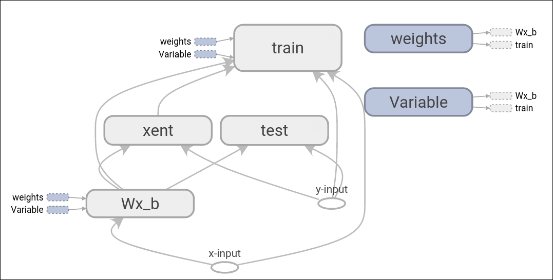
A simple data flow graph representation, as drawn on TensorBoard
A data flow graph is, succinctly, a complete TensorFlow computation, represented as a graph where nodes are operations and edges are data flowing between operations.
Normally, nodes implement mathematical operations, but also represent a connection to feed in data or a variable, or push out results.
Edges describe the input/output relationships between nodes. These data edges exclusively transport tensors. Nodes are assigned to computational devices and execute asynchronously and in parallel once all the tensors on their incoming edges become available.
All operations have a name and represent an abstract computation (for example, matrix inverse or product).
The computation graph is normally built while the library user creates the tensors and operations the model will support, so there is no need to build a Graph() object directly. The Python tensor constructors, such as tf.constant(), will add the necessary element to the default graph. The same occurs for TensorFlow operations.
For example, c = tf.matmul(a, b) creates an operation of MatMul type that takes tensors a and b as input and produces c as output.
tf.Operation.type: Returns the type of the operation (for example,MatMul)tf.Operation.inputs: Returns the list of tensor objects representing the operation's inputstf.Graph.get_operations(): Returns the list of operations in the graphtf.Graph.version: Returns the graph's autonumeric version
TensorFlow also provides a feed mechanism for patching a tensor directly into any operation in the graph.
A feed temporarily replaces the output of an operation with a tensor value. You supply feed data as an argument to a run()call. The feed is only used for the run call to which it is passed. The most common use case involves designating specific operations to be feed operations by using tf.placeholder() to create them.
In most computations, a graph is executed multiple times. Most tensors do not survive past a single execution of the graph. However, a variable is a special kind of operation that returns a handle to a persistent, mutable tensor that survives across executions of a graph. For machine learning applications of TensorFlow, the parameters of the model are typically stored in tensors held in variables, and are updated when running the training graph for the model.
Data flow graphs are written using Google's protocol buffers, so they can be read afterwards in a good variety of languages.
Protocol buffers are a language-neutral, platform-neutral, extensible mechanism for serializing structured data. You define the data structure first, and then you can use specialized generated code to read and write it with a variety of languages.
In this example we will build a very simple data flow graph, and observe an overview of the generated protobuffer file:
import tensorflow as tf
g = tf.Graph()
with g.as_default():
import tensorflow as tf
sess = tf.Session()
W_m = tf.Variable(tf.zeros([10, 5]))
x_v = tf.placeholder(tf.float32, [None, 10])
result = tf.matmul(x_v, W_m)
print g.as_graph_def()
The generated protobuffer (summarized) reads:
node {
  name: "zeros"
  op: "Const"
  attr {
    key: "dtype"
    value {
      type: DT_FLOAT
    }
  }
  attr {
    key: "value"
    value {
      tensor {
        dtype: DT_FLOAT
        tensor_shape {
          dim {
            size: 10
          }
          dim {
            size: 5
          }
        }
        float_val: 0.0
      }
    }
  }
}
...
node {
  name: "MatMul"
  op: "MatMul"
  input: "Placeholder"
  input: "Variable/read"
  attr {
    key: "T"
    value {
      type: DT_FLOAT
    }
  }
...
}
versions {
  producer: 8
}Client programs interact with the TensorFlow system by creating a Session. The Session object is a representation of the environment in which the computation will run. The Session object starts empty, and when the programmer creates the different operations and tensors, they will be added automatically to the Session, which will do no computation until the Run() method is called.
The Run() method takes a set of output names that need to be computed, as well as an optional set of tensors to be fed into the graph in place of certain outputs of nodes.
If we call this method, and there are operations on which the named operation depends, the Session object will execute all of them, and then proceed to execute the named one.
This simple line is the only one needed to create a Session:
s = tf.Session()
Sample command line output:
tensorflow/core/common_runtime/local_session.cc:45]Localsessioninteropparallelism threads:6
In this section we will be exploring some basic methods supported by TensorFlow. They are useful for initial data exploration and for preparing the data for better parallel computation.
TensorFlow supports many of the more common matrix operations, such as transpose, multiplication, getting the determinant, and inverse.
Here is a little example of those functions applied to sample data:
In [1]: import tensorflow as tf
In [2]: sess = tf.InteractiveSession()
In [3]: x = tf.constant([[2, 5, 3, -5],
...:                  [0, 3,-2,  5],
...:                  [4, 3, 5,  3],
...:                  [6, 1, 4,  0]])

In [4]: y = tf.constant([[4, -7, 4, -3, 4],
...:                  [6, 4,-7,  4, 7],
...:                  [2, 3, 2,  1, 4],
...:                  [1, 5, 5,  5, 2]])
In [5]: floatx = tf.constant([[2., 5., 3., -5.],
...:                       [0., 3.,-2.,  5.],
...:                       [4., 3., 5.,  3.],
...:                       [6., 1., 4.,  0.]])
In [6]: tf.transpose(x).eval() # Transpose matrix
Out[6]:
array([[ 2,  0,  4,  6],
[ 5,  3,  3,  1],
[ 3, -2,  5,  4],
[-5,  5,  3,  0]], dtype=int32)

In [7]: tf.matmul(x, y).eval() # Matrix multiplication
Out[7]:
array([[ 39, -10, -46,  -8,  45],
[ 19,  31,   0,  35,  23],
[ 47,  14,  20,  20,  63],
[ 38, -26,  25, -10,  47]], dtype=int32)

In [8]: tf.matrix_determinant(floatx).eval() # Matrix determinant
Out[8]: 818.0

In [9]: tf.matrix_inverse(floatx).eval() # Matrix inverse
Out[9]:
array([[-0.00855745,  0.10513446, -0.18948655,  0.29584351],
[ 0.12958434,  0.12224938,  0.01222495, -0.05134474],
[-0.01955992, -0.18826403,  0.28117359, -0.18092911],
[-0.08557458,  0.05134474,  0.10513448, -0.0415648 ]], dtype=float32)

In [10]: tf.matrix_solve(floatx, [[1],[1],[1],[1]]).eval() # Solve Matrix system
Out[10]:
array([[ 0.20293398],
[ 0.21271393],
[-0.10757945],
[ 0.02933985]], dtype=float32)
Reduction is an operation that applies an operation across one of the tensor's dimensions, leaving it with one less dimension.
The supported operations include (with the same parameters) product, minimum, maximum, mean, all, any, and accumulate_n).
In [1]: import tensorflow as tf

In [2]: sess = tf.InteractiveSession()
In [3]: x = tf.constant([[1,  2, 3],
...:                  [3,  2, 1],
...:                  [-1,-2,-3]])
In [4]:

In [4]: boolean_tensor = tf.constant([[True,  False, True],
...:                  [False, False, True],
...:                  [True, False, False]])

In [5]: tf.reduce_prod(x, reduction_indices=1).eval() # reduce prod
Out[5]: array([ 6,  6, -6], dtype=int32)

In [6]: tf.reduce_min(x, reduction_indices=1).eval() # reduce min
Out[6]: array([ 1,  1, -3], dtype=int32)

In [7]: tf.reduce_max(x, reduction_indices=1).eval() # reduce max
Out[7]: array([ 3,  3, -1], dtype=int32)

In [8]: tf.reduce_mean(x, reduction_indices=1).eval() # reduce mean
Out[8]: array([ 2,  2, -2], dtype=int32)

In [9]: tf.reduce_all(boolean_tensor, reduction_indices=1).eval() # reduce all
Out[9]: array([False, False, False], dtype=bool)

In [10]: tf.reduce_any(boolean_tensor, reduction_indices=1).eval() # reduce any
Out[10]: array([ True,  True,  True], dtype=bool)
Tensor segmentation is a process in which one of the dimensions is reduced, and the resulting elements are determined by an index row. If some elements in the row are repeated, the corresponding index goes to the value in it, and the operation is applied between the indexes with repeated indexes.
The index array size should be the same as the size of dimension 0 of the index array, and they must increase by one.
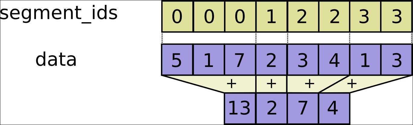
Segmentation explanation (redo)
In [1]: import tensorflow as tf
In [2]: sess = tf.InteractiveSession()
In [3]: seg_ids = tf.constant([0,1,1,2,2]); # Group indexes : 0|1,2|3,4
In [4]: tens1 = tf.constant([[2, 5, 3, -5],
...:                     [0, 3,-2,  5],
...:                     [4, 3, 5,  3],
...:                     [6, 1, 4,  0],
...:                     [6, 1, 4,  0]])  # A sample constant matrix

In [5]: tf.segment_sum(tens1, seg_ids).eval()   # Sum segmentation
Out[5]:
array([[ 2,  5,  3, -5],
[ 4,  6,  3,  8],
[12,  2,  8,  0]], dtype=int32)

In [6]: tf.segment_prod(tens1, seg_ids).eval() # Product segmentation
Out[6]:
array([[  2,   5,   3,  -5],
[  0,   9, -10,  15],
[ 36,   1,  16,   0]], dtype=int32)

In [7]: tf.segment_min(tens1, seg_ids).eval() # minimun value goes to group
Out[7]:
array([[ 2,  5,  3, -5],
[ 0,  3, -2,  3],
[ 6,  1,  4,  0]], dtype=int32)

In [8]: tf.segment_max(tens1, seg_ids).eval() # maximum value goes to group
Out[8]:
array([[ 2,  5,  3, -5],
[ 4,  3,  5,  5],
[ 6,  1,  4,  0]], dtype=int32)

In [9]: tf.segment_mean(tens1, seg_ids).eval() # mean value goes to group
Out[9]:
array([[ 2,  5,  3, -5],
[ 2,  3,  1,  4],
[ 6,  1,  4,  0]], dtype=int32)
Sequence utilities include methods such as argmin and argmax (showing the minimum and maximum value of a dimension), listdiff (showing the complement of the intersection between lists), where (showing the index of the true values on a tensor), and unique (showing unique values on a list).
In [1]: import tensorflow as tf
In [2]: sess = tf.InteractiveSession()
In [3]: x = tf.constant([[2, 5, 3, -5],
...:                  [0, 3,-2,  5],
...:                  [4, 3, 5,  3],
...:                  [6, 1, 4,  0]])
In [4]: listx = tf.constant([1,2,3,4,5,6,7,8])
In [5]: listy = tf.constant([4,5,8,9])

In [6]:

In [6]: boolx = tf.constant([[True,False], [False,True]])

In [7]: tf.argmin(x, 1).eval() # Position of the maximum value of columns
Out[7]: array([3, 2, 1, 3])

In [8]: tf.argmax(x, 1).eval() # Position of the minimum value of rows
Out[8]: array([1, 3, 2, 0])

In [9]: tf.listdiff(listx, listy)[0].eval() # List differences
Out[9]: array([1, 2, 3, 6, 7], dtype=int32)

In [10]: tf.where(boolx).eval() # Show true values
Out[10]:
array([[0, 0],
[1, 1]])

In [11]: tf.unique(listx)[0].eval() # Unique values in list
Out[11]: array([1, 2, 3, 4, 5, 6, 7, 8], dtype=int32)
These kinds of functions are related to a matrix shape.They are used to adjust unmatched data structures and to retrieve quick information about the measures of data. This can be useful when deciding a processing strategy at runtime.
In the following examples, we will start with a rank two tensor and will print some information about it.
Then we'll explore the operations that modify the matrix dimensionally, be it adding or removing dimensions, such as squeeze and expand_dims:
In [1]: import tensorflow as tf
In [2]: sess = tf.InteractiveSession()
In [3]: x = tf.constant([[2, 5, 3, -5],
...:                  [0, 3,-2,  5],
...:                  [4, 3, 5,  3],
...:                  [6, 1, 4,  0]])

In [4]: tf.shape(x).eval() # Shape of the tensor
Out[4]: array([4, 4], dtype=int32)

In [5]: tf.size(x).eval() # size of the tensor
Out[5]: 16

In [6]: tf.rank(x).eval() # rank of the tensor
Out[6]: 2

In [7]: tf.reshape(x, [8, 2]).eval() # converting to a 10x2 matrix
Out[7]:
array([[ 2,  5],
[ 3, -5],
[ 0,  3],
[-2,  5],
[ 4,  3],
[ 5,  3],
[ 6,  1],
[ 4,  0]], dtype=int32)

In [8]: tf.squeeze(x).eval() #  squeezing
Out[8]:
array([[ 2,  5,  3, -5],
[ 0,  3, -2,  5],
[ 4,  3,  5,  3],
[ 6,  1,  4,  0]], dtype=int32)

In [9]: tf.expand_dims(x,1).eval() #Expanding dims
Out[9]:
array([[[ 2,  5,  3, -5]],
[[ 0,  3, -2,  5]],
[[ 4,  3,  5,  3]],
[[ 6,  1,  4,  0]]], dtype=int32)
In order to extract and merge useful information from big datasets, the slicing and joining methods allow you to consolidate the required column information without having to occupy memory space with nonspecific information.
In the following examples, we'll extract matrix slices, split them, add padding, and pack and unpack rows:
In [1]: import tensorflow as tf
In [2]: sess = tf.InteractiveSession()
In [3]: t_matrix = tf.constant([[1,2,3],
...:                         [4,5,6],
...:                         [7,8,9]])
In [4]: t_array = tf.constant([1,2,3,4,9,8,6,5])
In [5]: t_array2= tf.constant([2,3,4,5,6,7,8,9])

In [6]: tf.slice(t_matrix, [1, 1], [2,2]).eval() # cutting an slice
Out[6]:
array([[5, 6],
[8, 9]], dtype=int32)

In [7]: tf.split(0, 2, t_array) # splitting the array in two
Out[7]:
[<tf.Tensor 'split:0' shape=(4,) dtype=int32>,
<tf.Tensor 'split:1' shape=(4,) dtype=int32>]

In [8]: tf.tile([1,2],[3]).eval() # tiling this little tensor 3 times
Out[8]: array([1, 2, 1, 2, 1, 2], dtype=int32)

In [9]: tf.pad(t_matrix, [[0,1],[2,1]]).eval() # padding
Out[9]:
array([[0, 0, 1, 2, 3, 0],
[0, 0, 4, 5, 6, 0],
[0, 0, 7, 8, 9, 0],
[0, 0, 0, 0, 0, 0]], dtype=int32)

In [10]: tf.concat(0, [t_array, t_array2]).eval() #concatenating list
Out[10]: array([1, 2, 3, 4, 9, 8, 6, 5, 2, 3, 4, 5, 6, 7, 8, 9], dtype=int32)

In [11]: tf.pack([t_array, t_array2]).eval() # packing
Out[11]:
array([[1, 2, 3, 4, 9, 8, 6, 5],
[2, 3, 4, 5, 6, 7, 8, 9]], dtype=int32)

In [12]: sess.run(tf.unpack(t_matrix)) # Unpacking, we need the run method to view the tensors
Out[12]:
[array([1, 2, 3], dtype=int32),
array([4, 5, 6], dtype=int32),
array([7, 8, 9], dtype=int32)]

In [13]: tf.reverse(t_matrix, [False,True]).eval() # Reverse matrix
Out[13]:
array([[3, 2, 1],
[6, 5, 4],
[9, 8, 7]], dtype=int32)
Visualizing summarized information is a vital part of any data scientist's toolbox.
TensorBoard is a software utility that allows the graphical representation of the data flow graph and a dashboard used for the interpretation of results, normally coming from the logging utilities:
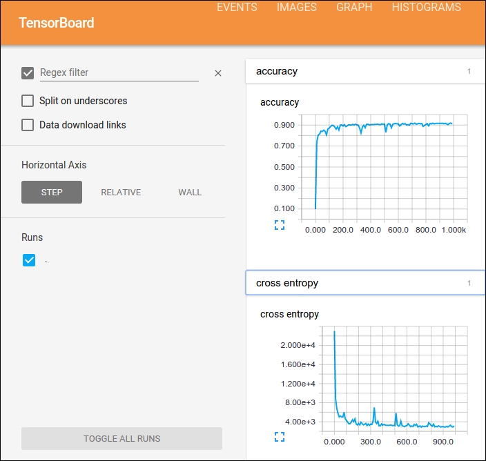
TensorBoard GUI
All the tensors and operations of a graph can be set to write information to logs. TensorBoard analyzes that information, written normally, while the Session is running, and presents the user with many graphical items, one for each graph item.
Every computation graph we build, TensorFlow has a real-time logging mechanism for, in order to save almost all the information that a model possesses.
However, the model builder has to take into account which of the possible hundred information dimensions it should save, to later serve as an analysis tool.
To save all the required information, TensorFlow API uses data output objects, called Summaries.
These Summaries write results into TensorFlow event files, which gather all the required data generated during a Session's run.
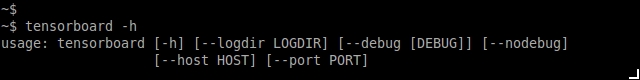
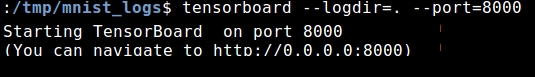
In the following example, we'll running TensorBoard directly on a generated event log directory:
All Summaries in a TensorFlow Session are written by a SummaryWriter object. The main method to call is:
tf.train.SummaryWriter.__init__(logdir, graph_def=None)
This command will create a SummaryWriter and an event file, in the path of the parameter.
The constructor of the the SummaryWriter will create a new event file in logdir. This event file will contain Event type protocol buffers constructed when you call one of the following functions: add_summary(), add_session_log(), add_event(), or add_graph().
If you pass a graph_def protocol buffer to the constructor, it is added to the event file. (This is equivalent to calling add_graph() later).
When you run TensorBoard, it will read the graph definition from the file and display it graphically so you can interact with it.
First, create the TensorFlow graph that you'd like to collect summary data from and decide which nodes you would like to annotate with summary operations.
Operations in TensorFlow don't do anything until you run them, or an operation that depends on their output. And the summary nodes that we've just created are peripheral to your graph: none of the ops you are currently running depend on them. So, to generate summaries, we need to run all of these summary nodes. Managing them manually would be tedious, so use tf.merge_all_summaries to combine them into a single op that generates all the summary data.
Then, you can just run the merged summary op, which will generate a serialized Summary protobuf object with all of your summary data at a given step. Finally, to write this summary data to disk, pass the Summary protobuf to a tf.train.SummaryWriter.
The SummaryWriter takes a logdir in its constructor, this logdir is quite important, it's the directory where all of the events will be written out. Also, the SummaryWriter can optionally take a GraphDef in its constructor. If it receives one, then TensorBoard will visualize your graph as well.
Now that you've modified your graph and have a SummaryWriter, you're ready to start running your network! If you want, you could run the merged summary op every single step, and record a ton of training data. That's likely to be more data than you need, though. Instead, consider running the merged summary op every n steps.
This is a list of the different Summary types, and the parameters employed on its construction:
tf.scalar_summary(tag, values, collections=None, name=None)tf.image_summary(tag, tensor, max_images=3, collections=None, name=None)tf.histogram_summary(tag, values, collections=None, name=None)
These are special functions, that are used to merge the values of different operations, be it a collection of summaries, or all summaries in a graph:
tf.merge_summary(inputs, collections=None, name=None)tf.merge_all_summaries(key='summaries')
Finally, as one last aid to legibility, the visualization uses special icons for constants and summary nodes. To summarize, here's a table of node symbols:
|
Symbol |
Meaning |
|

|
High-level node representing a name scope. Double-click to expand a high-level node. |
|

|
Sequence of numbered nodes that are not connected to each other. |
|

|
Sequence of numbered nodes that are connected to each other. |
|

|
An individual operation node. |
|

|
A constant. |
|

|
A summary node. |
|

|
Edge showing the data flow between operations. |
|

|
Edge showing the control dependency between operations. |
|

|
A reference edge showing that the outgoing operation node can mutate the incoming tensor. |
Navigate the graph by panning and zooming. Click and drag to pan, and use a scroll gesture to zoom. Double-click on a node, or click on its + button, to expand a name scope that represents a group of operations. To easily keep track of the current viewpoint when zooming and panning, there is a minimap in the bottom-right corner:
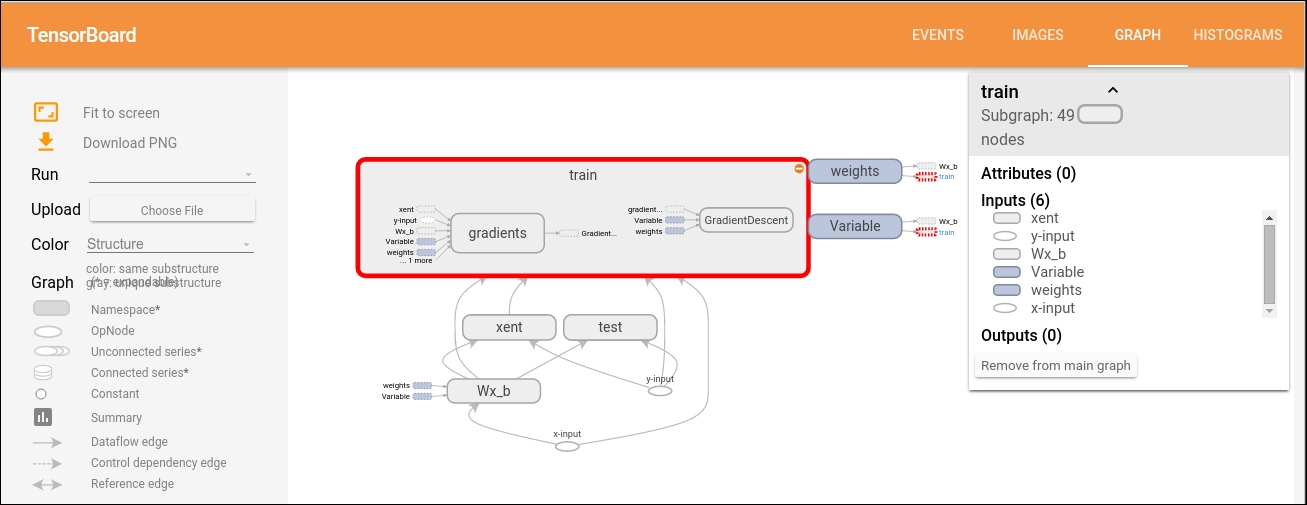
Openflow with one expanded operations group and legends
To close an open node, double-click it again or click its - button. You can also click once to select a node. It will turn a darker color, and details about it and the nodes it connects to will appear in the info card in the upper-right corner of the visualization.
Selection can also be helpful in understanding high-degree nodes. Select any high-degree node, and the corresponding node icons for its other connections will be selected as well. This makes it easy, for example, to see which nodes are being saved and which aren't.
Clicking on a node name in the info card will select it. If necessary, the viewpoint will automatically pan so that the node is visible.
Finally, you can choose two color schemes for your graph, using the color menu above the legend. The default Structure View shows the structure: when two high-level nodes have the same structure, they appear in the same color of the rainbow. Uniquely structured nodes are gray. There's a second view, which shows what device the different operations run on. Name scopes are colored proportionally, to the fraction of devices for the operations inside them.
TensorFlow reads a number of the most standard formats, including the well-known CSV, image files (JPG and PNG decoders), and the standard TensorFlow format.
For reading the well-known CSV format, TensorFlow has its own methods. In comparison with other libraries, such as pandas, the process to read a simple CSV file is somewhat more complicated.
The reading of a CSV file requires a couple of the previous steps. First, we must create a filename queue object with the list of files we'll be using, and then create a TextLineReader. With this line reader, the remaining operation will be to decode the CSV columns, and save it on tensors. If we want to mix homogeneous data together, the pack method will work.
The Iris flower dataset or Fisher's Iris dataset is a well know benchmark for classification problems. It's a multivariate data set introduced by Ronald Fisher in his 1936 paper The use of multiple measurements in taxonomic problems as an example of linear discriminant analysis.
The data set consists of 50 samples from each of three species of Iris (Iris setosa, Iris virginica, and Iris versicolor). Four features were measured in each sample: the length and the width of the sepals and petals, in centimeters. Based on the combination of these four features, Fisher developed a linear discriminant model to distinguish the species from each other. (You'll be able to get the .csv file for this dataset in the code bundle of the book.)
In order to read the CSV file, you will have to download it and put it in the same directory as where the Python executable is running.
In the following code sample, we'll be reading and printing the first five records from the well-known Iris database:
import tensorflow as tf
sess = tf.Session()
filename_queue = tf.train.string_input_producer(
tf.train.match_filenames_once("./*.csv"),
shuffle=True)
reader = tf.TextLineReader(skip_header_lines=1)
key, value = reader.read(filename_queue)
record_defaults = [[0.], [0.], [0.], [0.], [""]]
col1, col2, col3, col4, col5 = tf.decode_csv(value, record_defaults=record_defaults)  # Convert CSV records to tensors. Each column maps to one tensor.
features = tf.pack([col1, col2, col3, col4])

tf.initialize_all_variables().run(session=sess)
coord = tf.train.Coordinator()
threads = tf.train.start_queue_runners(coord=coord, sess=sess)

for iteration in range(0, 5):
 example = sess.run([features])
 print(example)
 coord.request_stop()
 coord.join(threads)
And this is how the output would look:
TensorFlow allows importing data from image formats, it will really be useful for importing custom image inputs for image oriented models.The accepted image formats will be JPG and PNG, and the internal representation will be uint8 tensors, one rank two tensor for each image channel:
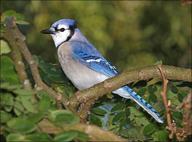
Sample image to be read
In this example, we will load a sample image and apply some additional processing to it, saving the resulting images in separate files:
import tensorflow as tf
sess = tf.Session()
filename_queue = tf.train.string_input_producer(tf.train.match_filenames_once("./blue_jay.jpg"))
reader = tf.WholeFileReader()
key, value = reader.read(filename_queue)
image=tf.image.decode_jpeg(value)
flipImageUpDown=tf.image.encode_jpeg(tf.image.flip_up_down(image))
flipImageLeftRight=tf.image.encode_jpeg(tf.image.flip_left_right(image))
tf.initialize_all_variables().run(session=sess)
coord = tf.train.Coordinator()
threads = tf.train.start_queue_runners(coord=coord, sess=sess)
example = sess.run(flipImageLeftRight)
print example
file=open ("flippedUpDown.jpg", "wb+")
file.write (flipImageUpDown.eval(session=sess))
file.close()
file=open ("flippedLeftRight.jpg", "wb+")
file.write (flipImageLeftRight.eval(session=sess))
file.close()
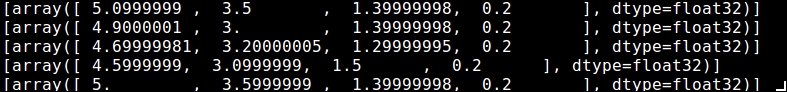
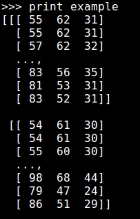
The print example line will show a line-by-line summary of the RGB values in the image:
The final images will look like:
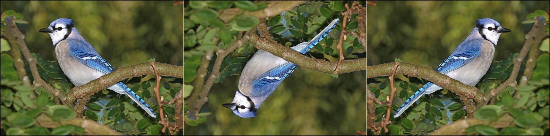
Original and altered images compared (flipUpDown and flipLeftRight)
Another approach is to convert the arbitrary data you have, into the official format. This approach makes it easier to mix and match data sets and network architectures.
You can write a little program that gets your data, stuffs it in an example protocol buffer, serializes the protocol buffer to a string, and then writes the string to a TFRecords file using the tf.python_io.TFRecordWriter class.
To read a file of TFRecords, use tf.TFRecordReader with the tf.parse_single_example decoder. The parse_single_example
op decodes the example protocol buffers into tensors.
In this chapter we have learned the main data structures and simple operations we can apply to data, and a succinct summary of the parts of a computational graph.
These kinds of operations will be the foundation for the forthcoming techniques. They allow the data scientist to decide on simpler models if the separation of classes or the adjusting functions look sufficiently clear, or to advance directly to much more sophisticated tools, having looked at the overall characteristics of the current data.
In the next chapter, we will begin building and running graphs, and will solve problems using some of the methods found in this chapter.

