


The 21st century is the digital century, where every person on every rung of the economic ladder is using digital devices and producing data in digital format at an unprecedented rate. 90% of data generated in the last 10 years was generated in the last 2 years. This is an exponential rate of growth, where the amount of data is increasing by 10 times every 2 years. This trend is expected to continue for the foreseeable future:

Figure 1.1: The increase in digital data year on year
But this data is not just stored in hard drives; it's being used to make lives better. For example, Google uses the data it has to serve you better results, and Netflix uses the data it has to serve you better movie recommendations. In fact, their decision to make their hit show House of Cards was based on analytics. IBM is using the medical data it has to create an artificially intelligent doctor and to detect cancerous tumors from x-ray images.
To process this amount of data with computers and come up with relevant results, a particular class of algorithms is used. These algorithms are collectively known as machine learning algorithms. Machine learning is divided into two parts, depending on the type of data that is being used: one is called supervised learning and the other is called unsupervised learning.
Supervised learning is done when we get labeled data. For example, say we get 1,000 images of x-rays from a hospital that are labeled as normal or fractured. We can use this data to train a machine learning model to predict whether an x-ray image shows a fractured bone or not.
Unsupervised learning is when we just have raw data and are expected to come up with insights without any labels. We have the ability to understand the data and recognize patterns in it without explicitly being told what patterns to identify. By the end of this book, you're going to be aware of all of the major types of unsupervised learning algorithms. In this book, we're going to be using the R programming language for demonstration, but the algorithms are the same for all languages.
In this chapter, we're going to study the most basic type of unsupervised learning, clustering. At first, we're going to study what clustering is, its types, and how to create clusters with any type of dataset. Then we're going to study how each type of clustering works, looking at their advantages and disadvantages. At the end, we're going to learn when to use which type of clustering.
Clustering is a set of methods or algorithms that are used to find natural groupings according to predefined properties of variables in a dataset. The Merriam-Webster dictionary defines a cluster as "a number of similar things that occur together." Clustering in unsupervised learning is exactly what it means in the traditional sense. For example, how do you identify a bunch of grapes from far away? You have an intuitive sense without looking closely at the bunch whether the grapes are connected to each other or not. Clustering is just like that. An example of clustering is presented here:

Figure 1.2: A representation of two clusters in a dataset
In the preceding graph, the data points have two properties: cholesterol and blood pressure. The data points are classified into two clusters, or two bunches, according to the Euclidean distance between them. One cluster contains people who are clearly at high risk of heart disease and the other cluster contains people who are at low risk of heart disease. There can be more than two clusters, too, as in the following example:

Figure 1.3: A representation of three clusters in a dataset
In the preceding graph, there are three clusters. One additional group of people has high blood pressure but with low cholesterol. This group may or may not have a risk of heart disease. In further sections, clustering will be illustrated on real datasets in which the x and y coordinates denote actual quantities.
Like all methods of unsupervised learning, clustering is mostly used when we don't have labeled data – data with predefined classes – for training our models. Clustering uses various properties, such as Euclidean distance and Manhattan distance, to find patterns in the data and classify them according to similarities in their properties without having any labels for training. So, clustering has many use cases in fields where labeled data is unavailable or we want to find patterns that are not defined by labels.
The following are some applications of clustering:
Exploratory data analysis: When we have unlabeled data, we often do clustering to explore the underlying structure and categories of the dataset. For example, a retail store might want to explore how many different segments of customers they have, based on purchase history.
Generating training data: Sometimes, after processing unlabeled data with clustering methods, it can be labeled for further training with supervised learning algorithms. For example, two different classes that are unlabeled might form two entirely different clusters, and using their clusters, we can label data for further supervised learning algorithms that are more efficient in real-time classification than our unsupervised learning algorithms.
Recommender systems: With the help of clustering, we can find the properties of similar items and use these properties to make recommendations. For example, an e-commerce website, after finding customers in the same clusters, can recommend items to customers in that cluster based upon the items bought by other customers in that cluster.
Natural language processing: Clustering can be used for the grouping of similar words, texts, articles, or tweets, without labeled data. For example, you might want to group articles on the same topic automatically.
Anomaly detection: You can use clustering to find outliers. We're going to learn about this in Chapter 6, Anomaly Detection. Anomaly detection can also be used in cases where we have unbalanced classes in data, such as in the case of the detection of fraudulent credit card transactions.
In this chapter, we're going to use the Iris flowers dataset in exercises to learn how to classify three species of Iris flowers (Versicolor, Setosa, and Virginica) without using labels. This dataset is built-in to R and is very good for learning about the implementation of clustering techniques.
Note that in our exercise dataset, we have final labels for the flowers. We're going to compare clustering results with those labels. We choose this dataset just to demonstrate that the results of clustering make sense. In the case of datasets such as the wholesale customer dataset (covered later in the book), where we don't have final labels, the results of clustering cannot be objectively verified and therefore might lead to misguided conclusions. That's the kind of use case where clustering is used in real life when we don't have final labels for the dataset. This point will be clearer once you have done both the exercises and activities.
In this exercise, we're going to learn how to use the Iris dataset in R. Assuming you already have R installed in your system, let's proceed:
Load the Iris dataset into a variable as follows:
iris_data<-iris
Now that our Iris data is in the iris_data variable, we can have a look at its first few rows by using the head function in R:
head(iris_data)
The output is as follows:

Figure 1.4: The first six rows of the Iris dataset
We can see our dataset has five columns. We're mostly going to use two columns for ease of visualization in plots of two dimensions.
As stated previously, clustering algorithms find natural groupings in data. There are many ways in which we can find natural groupings in data. The following are the methods that we're going to study in this chapter:
k-means clustering
k-medoids clustering
Once the concepts related to the basic types of clustering are clear, we will have a look at other types of clustering, which are as follows:
k-modes
Density-based clustering
Agglomerative hierarchical clustering
Divisive clustering
K-means clustering is one of the most basic types of unsupervised learning algorithm. This algorithm finds natural groupings in accordance with a predefined similarity or distance measure. The distance measure can be any of the following:
Euclidean distance
Manhattan distance
Cosine distance
Hamming distance
To understand what a distance measure does, take the example of a bunch of pens. You have 12 pens. Six of them are blue, and six red. Six of them are ball point pens and six are ink pens. If you were to use ink color as a similarity measure, then six blue pens and six red pens will be in different clusters. The six blue pens can be ink or ball point here; there's no restriction on that. But if you were to use the type of pen as the similarity measure, then the six ink pens and six ball point pens would be in different clusters. Now it doesn't matter whether the pens in each cluster are of the same color or not.
Euclidean distance is the straight-line distance between any two points. Calculation of this distance in two dimensions can be thought of an extension of the Pythagorean theorem, which you might have studied in school. But Euclidean distance can be calculated between two points in any n-dimensional space, not just a two-dimensional space. The Euclidean distance between any two points is the square root of the sum of squares of differences between the coordinates. An example of the calculation of Euclidean distance is presented here:

Figure 1.5: Representation of Euclidean distance calculation
In k-means clustering, Euclidean distance is used. One disadvantage of using Euclidean distance is that it loses its meaning when the dimensionality of data is very high. This is related to a phenomenon known as the curse of dimensionality. When datasets possess many dimensions, they can be harder to work with, since distances between all points can become extremely high, and the distances are difficult to interpret and visualize.
So, when the dimensionality of data is very high, either we reduce its dimensions with principal component analysis, which we're going to study in Chapter 4, Dimension Reduction, or we use cosine similarity.
By definition, Manhattan distance is the distance between two points measured along a right angle to the axes:

Figure 1.6: Representation of Manhattan distance
The length of the diagonal line is the Euclidean distance between the two points. Manhattan distance is simply the sum of the absolute value of the differences between two coordinates. So, the main difference between Euclidean distance and Manhattan distance is that with Euclidean distance, we square the distances between coordinates and then take the root of the sum, but in Manhattan distance, we directly take the sum of the absolute value of the differences between coordinates.
Cosine similarity between any two points is defined as the cosine of the angle between any two points with the origin as its vertex. It can be calculated by dividing the dot product of any two vectors by the product of the magnitudes of the vectors:

Figure 1.7: Representation of cosine similarity and cosine distance
Cosine distance is defined as (1-cosine similarity).
Cosine distance varies from 0 to 2, whereas cosine similarity varies between -1 to 1. Always remember that cosine similarity is one minus the value of of the cosine distance.
The Hamming distance is a special type of distance that is used for categorical variables. Given two points of equal dimensions, the Hamming distance is defined as the number of coordinates differing from one another. For example, let's take two points, (0, 1, 1) and (0, 1, 0). Only one value, which is the last value, is different between these two variables. As such, the Hamming distance between them is 1:

Figure 1.8: Representation of the Hamming distance
K-means clustering is used to find clusters in a dataset of similar points when we have unlabeled data. In this chapter, we're going to use the Iris flowers dataset. This dataset contains information about the length and breadth of sepals and petals of flowers of different species. With the help of unsupervised learning, we're going to learn how to differentiate between them without knowing which properties belong to which species. The following is the scatter plot of our dataset:

Figure 1.9: A scatter plot of the Iris flowers dataset
This is the scatter plot of two variables of the Iris flower dataset: sepal length and sepal width.
If we were to identify the clusters in the preceding dataset according to the distance between the points, we would choose clusters that look like bunches of grapes hanging from a tree. You can see that there are two major bunches (one in the top left and the other being the remaining points). The k-means algorithm identifies these "bunches" of grapes.
The following figure shows the same scatter plot, but with the three different species of Iris shown in different colors. These species are taken from the 'species' column of the original dataset, and are as follows: Iris setosa (shown in green), Iris versicolor (shown in red), and Iris virginica (shown in blue). We're going to see whether we can determine these species by forming our own classifications using clustering:

Figure 1.10: A scatter plot showing different species of Iris flowers dataset
Here is a photo of Iris setosa, which is represented in green in the preceding scatter plot:

Figure 1.11: Iris setosa
The following is a photo of Iris versicolor, which is represented in red in the preceding scatter plot:

Figure 1.12: Iris versicolor
Here is a photo of Iris virginica, which is represented in blue in the preceding scatter plot:

Figure 1.13: Iris virginica
As we saw in the scatter plot in figure 1.9, each data point represents a flower. We're going to find clusters that will identify these species. To do this type of clustering, we're going to use k-means clustering, where k is the number of clusters we want. The following are the steps to perform k-means clustering, which, for simplicity of understanding, we're going to demonstrate with two clusters. We will build up to using three clusters later, in order to try and match the actual species groupings:
Choose any two random coordinates, k1 and k2, on the scatter plot as initial cluster centers.
Calculate the distance of each data point in the scatter plot from coordinates k1 and k2.
Assign each data point to a cluster based on whether it is closer to k1 or k2
Find the mean coordinates of all points in each cluster and update the values of k1 and k2 to those coordinates respectively.
Start again from Step 2 until the coordinates of k1 and k2 stop moving significantly, or after a certain pre-determined number of iterations of the process.
We're going to demonstrate the preceding algorithm with graphs and code.
In this exercise, we will implement k-means clustering step by step:
Load the built-in Iris dataset in the iris_data variable:
iris_data<-iris
Set the color for different species for representation on the scatter plot. This will help us see how the three different species are split between our initial two groupings:
iris_data$t_color='red'
iris_data$t_color[which(iris_data$Species=='setosa')]<-'green'
iris_data$t_color[which(iris_data$Species=='virginica')]<-'blue'
Choose any two random clusters' centers to start with:
k1<-c(7,3)
k2<-c(5,3)
Plot the scatter plot along with the centers you chose in the previous step. Pass the length and width of the sepals of the iris flowers, along with the color, to the plot function in the first line, and then pass x and y coordinates of both the centers to the points() function. Here, pch is for selecting the type of representation of the center of the clusters – in this case, 4 is a cross and 5 is a diamond:
plot(iris_data$Sepal.Length,iris_data$Sepal.Width,col=iris_data$t_color)
points(k1[1],k1[2],pch=4)
points(k2[1],k2[2],pch=5)
The output is as follows:

Figure 1.14: A scatter plot of the chosen cluster centers
Choose the number of iterations you want. The number of iterations should be such that the centers stop changing significantly after each iteration. In our case, six iterations are sufficient:
number_of_steps<-6
Initialize the variable that will keep track of the number of iterations in the loop:
n<-1
Start the while loop to find the final cluster centers:
while(n<number_of_steps)
{
Calculate the distance of each point from the current cluster centers, which is Step 2 in the algorithm. We're calculating the Euclidean distance here using the sqrt function:
  iris_data$distance_to_clust1 <- sqrt((iris_data$Sepal.Length-k1[1])^2+(iris_data$Sepal.Width-k1[2])^2)
  iris_data$distance_to_clust2 <- sqrt((iris_data$Sepal.Length-k2[1])^2+(iris_data$Sepal.Width-k2[2])^2)
Assign each point to the cluster whose center it is closest to, which is Step 3 of the algorithm:
  iris_data$clust_1 <- 1*(iris_data$distance_to_clust1<=iris_data$distance_to_clust2)
  iris_data$clust_2 <- 1*(iris_data$distance_to_clust1>iris_data$distance_to_clust2)
Calculate new cluster centers by calculating the mean x and y coordinates of the point in each cluster (step 4 in the algorithm) with the mean() function in R:
  k1[1]<-mean(iris_data$Sepal.Length[which(iris_data$clust_1==1)])
  k1[2]<-mean(iris_data$Sepal.Width[which(iris_data$clust_1==1)])
  k2[1]<-mean(iris_data$Sepal.Length[which(iris_data$clust_2==1)])
  k2[2]<-mean(iris_data$Sepal.Width[which(iris_data$clust_2==1)])
Update the variable that is keeping the count of iterations for us to effectively carry out step 5 of the algorithm:
  n=n+1
}
Now we're going to overwrite the species colors with new colors to demonstrate the two clusters. So, there will only be two colors on our next scatter plot – one color for cluster 1, and one color for cluster 2:
iris_data$color='red'
iris_data$color[which(iris_data$clust_2==1)]<-'blue'
Plot the new scatter plot, which contains clusters along with cluster centers:
plot(iris_data$Sepal.Length,iris_data$Sepal.Width,col=iris_data$color)
points(k1[1],k1[2],pch=4)
points(k2[1],k2[2],pch=5)
The output will be as follows:

Figure 1.15: A scatter plot representing each cluster with a different color
Notice how setosa (which used to be green) has been grouped in the left cluster, while most of the virginica flowers (which were blue) have been grouped into the right cluster. The versicolor flowers (which were red) have been split between the two new clusters.
You have successfully implemented the k-means clustering algorithm to identify two groups of flowers based on their sepal size. Notice how the position of centers has changed after running the algorithm.
In the following activity, we are going to increase the number of clusters to three to see whether we can group the flowers correctly into their three different species.
Write an R program to perform k-means clustering on the Iris dataset using three clusters. In this activity, we're going to perform the following steps:
Choose any three random coordinates, k1, k2, and k3, on the plot as centers.
Calculate the distance of each data point from k1, k2, and k3.
Classify each point by the cluster whose center it is closest to.
Find the mean coordinates of all points in the respective clusters and update the values of k1, k2, and k3 to those values.
Start again from Step 2 until the coordinates of k1, k2, and k3 stop moving significantly, or after 10 iterations of the process.
The outcome of this activity will be a chart with three clusters, as follows:

Figure 1.16: The expected scatter plot for the given cluster centers
You can compare your chart to Figure 1.10 to see how well the clusters match the actual species classifications.
In this section, we're going to use some built-in libraries of R to perform k-means clustering instead of writing custom code, which is lengthy and prone to bugs and errors. Using pre-built libraries instead of writing our own code has other advantages, too:
Library functions are computationally efficient, as thousands of man hours have gone into the development of those functions.
Library functions are almost bug-free as they've been tested by thousands of people in almost all practically-usable scenarios.
Using libraries saves time, as you don't have to invest time in writing your own code.
In the previous activity, we performed k-means clustering with three clusters by writing our own code. In this section, we're going to achieve a similar result with the help of pre-built R libraries.
At first, we're going to start with a distribution of three types of flowers in our dataset, as represented in the following graph:

Figure 1.17: A graph representing three species of iris in three colors
In the preceding plot, setosa is represented in blue, virginica in gray, and versicolor in pink.
With this dataset, we're going to perform k-means clustering and see whether the built-in algorithm is able to find a pattern on its own to classify these three species of iris using their sepal sizes. This time, we're going to use just four lines of code.
In this exercise, we're going to learn to do k-means clustering in a much easier way with the pre-built libraries of R. By completing this exercise, you will be able to divide the three species of Iris into three separate clusters:
We put the first two columns of the iris dataset, sepal length and sepal width, in the iris_data variable:
iris_data<-iris[,1:2]
We find the k-means cluster centers and the cluster to which each point belongs, and store it all in the km.res variable. Here, in the kmeans, function we enter the dataset as the first parameter, and the number of clusters we want as the second parameter:
km.res<-kmeans(iris_data,3)
Install the factoextra library as follows:
install.packages('factoextra')We import the factoextra library for visualization of the clusters we just created. Factoextra is an R package that is used for plotting multivariate data:
library("factoextra")Generate the plot of the clusters. Here, we need to enter the results of k-means as the first parameter. In data, we need to enter the data on which clustering was done. In pallete, we're selecting the type of the geometry of points, and in ggtheme, we're selecting the theme of the output plot:
fviz_cluster(km.res, data = iris_data,palette = "jco",ggtheme = theme_minimal())
The output will be as follows:

Figure 1.18: Three species of Iris have been clustered into three clusters
Here, if you compare Figure 1.18 to Figure 1.17, you will see that we have classified all three species almost correctly. The clusters we've generated don't exactly match the species shown in figure 1.18, but we've come very close considering the limitations of only using sepal length and width to classify them.
You can see from this example that clustering would've been a very useful way of categorizing the irises if we didn't already know their species. You will come across many examples of datasets where you don't have labeled categories, but are able to use clustering to form your own groupings.
Market segmentation is dividing customers into different segments based on common characteristics. The following are the uses of customer segmentation:
Increasing customer conversion and retention
Developing new products for a particular segment by identifying it and its needs
Improving brand communication with a particular segment
Identifying gaps in marketing strategy and making new marketing strategies to increase sales
In this exercise, we will have a look at the data in the wholesale customer dataset.
Note
For all the exercises and activities where we are importing an external CSV or image files, go to RStudio-> Session-> Set Working Directory-> To Source File Location. You can see in the console that the path is set automatically.
To download the CSV file, go to https://github.com/TrainingByPackt/Applied-Unsupervised-Learning-with-R/tree/master/Lesson01/Exercise04/wholesale_customers_data.csv. Click on wholesale_customers_data.csv.
Note
This dataset is taken from the UCI Machine Learning Repository. You can find the dataset at https://archive.ics.uci.edu/ml/machine-learning-databases/00292/. We have downloaded the file and saved it at https://github.com/TrainingByPackt/Applied-Unsupervised-Learning-with-R/tree/master/Lesson01/Exercise04/wholesale_customers_data.csv.
Save it to the folder in which you have installed R. Now, to load it in R, use the following function:
ws<-read.csv("wholesale_customers_data.csv")Now we may have a look at the different columns and rows in this dataset by using the following function in R:
head(ws)
The output is as follows:

Figure 1.19: Columns of the wholesale customer dataset
These six rows show the first six rows of annual spending in monetary units by category of product.
For this activity, we're going to use the wholesale customer dataset from the UCI Machine Learning Repository. It's available at: https://github.com/TrainingByPackt/Applied-Unsupervised-Learning-with-R/tree/master/Lesson01/Activity02/wholesale_customers_data.csv. We're going to identify customers belonging to different market segments who like to spend on different types of goods with clustering. Try k-means clustering for values of k from 2 to 6.
Note
This dataset is taken from the UCI Machine Learning Repository. You can find the dataset at https://archive.ics.uci.edu/ml/machine-learning-databases/00292/. We have downloaded the file and saved it at https://github.com/TrainingByPackt/Applied-Unsupervised-Learning-with-R/tree/master/Lesson01/Activity02/wholesale_customers_data.csv.
These steps will help you complete the activity:
Read data downloaded from the UCI Machine Learning Repository into a variable. The data can be found at: https://github.com/TrainingByPackt/Applied-Unsupervised-Learning-with-R/tree/master/Lesson01/Activity02/wholesale_customers_data.csv.
Select only two columns, Grocery and Frozen, for easy visualization of clusters.
As in Step 2 of Exercise 4, Exploring the Wholesale Customer Dataset, change the value for the number of clusters to 2 and generate the cluster centers.
Plot the graph as in Step 4 in Exercise 4, Exploring the Wholesale Customer Dataset.
Save the graph you generate.
Repeat Steps 3, 4, and 5 by changing value for the number of clusters to 3, 4, 5, and 6.
Decide which value for the number of clusters best classifies the dataset.
The output will be chart of six clusters as follows:
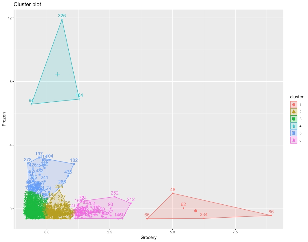
Figure 1.20: The expected chart for six clusters
k-medoids is another type of clustering algorithm that can be used to find natural groupings in a dataset. k-medoids clustering is very similar to k-means clustering, except for a few differences. The k-medoids clustering algorithm has a slightly different optimization function than k-means. In this section, we're going to study k-medoids clustering.
There are many different types of algorithms to perform k-medoids clustering, the simplest and most efficient of which is Partitioning Around Medoids, or PAM for short. In PAM, we do the following steps to find cluster centers:
Choose k data points from the scatter plot as starting points for cluster centers.
Calculate their distance from all the points in the scatter plot.
Classify each point into the cluster whose center it is closest to.
Select a new point in each cluster that minimizes the sum of distances of all points in that cluster from itself.
Repeat Step 2 until the centers stop changing.
You can see that the PAM algorithm is identical to the k-means clustering algorithm, except for Step 1 and Step 4. For most practical purposes, k-medoids clustering gives almost identical results to k-means clustering. But in some special cases where we have outliers in a dataset, k-medoids clustering is preferred as it's more robust to outliers. More about when to use which type of clustering and their differences will be studied in later sections.
In this section, we're going to use the same Iris flowers dataset that we used in the last two sections and compare to see whether the results are visibly different from the ones we got last time. Instead of writing code to perform each step of the k-medoids algorithm, we're directly going to use libraries of R to do PAM clustering.
In this exercise, we're going to perform k-medoids with R's pre-built libraries:
Store the first two columns of the iris dataset in the iris_data variable:
iris_data<-iris[,1:2]
Install the cluster package:
install.packages("cluster")Import the cluster package:
library("cluster")Store the PAM clustering results in the km.res variable:
km<-pam(iris_data,3)
Import the factoextra library:
library("factoextra")Plot the PAM clustering results in a graph:
fviz_cluster(km, data = iris_data,palette = "jco",ggtheme = theme_minimal())
The output is as follows:

Figure 1.21: Results of k-medoids clustering
The results of k-medoids clustering are not very different from those of the k-means clustering we did in the previous section.
So, we can see that the preceding PAM algorithm classifies our dataset into three clusters that are similar to the clusters we got with k-means clustering. If we plot the results of both types of clustering side by side, we can clearly see how similar they are:

Figure 1.22: The results of k-medoids clustering versus k-means clustering
In the preceding graphs, observe how the centers of both k-means and k-medoids clustering are so close to each other, but centers for k-medoids clustering are directly overlapping on points already in the data while the centers for k-means clustering are not.
Now that we've studied both k-means and k-medoids clustering, which are almost identical to each other, we're going to study the differences between them and when to use which type of clustering:
Computational complexity: Of the two methods, k-medoids clustering is computationally more expensive. When our dataset is too large (>10,000 points) and we want to save computation time, we'll prefer k-means clustering over k-medoids clustering.
Presence of outliers: k-means clustering is more sensitive to outliers than k-medoids. Cluster center positions can shift significantly due to the presence of outliers in the dataset, so we use k-medoids clustering when we have to build clusters resilient to outliers.
Cluster centers: Both the k-means and k-medoids algorithms find cluster centers in different ways. The center of a k-medoids cluster is always a data point in the dataset. The center of a k-means cluster does not need to be a data point in the dataset.
Use the Wholesale customer dataset to perform both k-means and k-medoids clustering, and then compare the results. Read the data downloaded from the UCI machine learning repository into a variable. The data can be found at https://github.com/TrainingByPackt/Applied-Unsupervised-Learning-with-R/tree/master/Lesson01/Data/wholesale_customers_data.csv.
Note
This dataset is taken from the UCI Machine Learning Repository. You can find the dataset at https://archive.ics.uci.edu/ml/machine-learning-databases/00292/. We have downloaded the file and saved it at https://github.com/TrainingByPackt/Applied-Unsupervised-Learning-with-R/tree/master/Lesson01/Activity03/wholesale_customers_data.csv.
These steps will help you complete the activity:
Select only two columns, Grocery and Frozen, for easy two-dimensional visualization of clusters.
Use k-medoids clustering to plot a graph showing four clusters for this data.
Use k-means clustering to plot a four-cluster graph.
Compare the two graphs to comment on how the results of the two methods differ.
The outcome will be a k-means plot of the clusters as follows:

Figure 1.23: The expected k-means plot of the cluster
Until now, we've been working on the iris flowers dataset, in which we know how many categories of flowers there are, and we chose to divide our dataset into three clusters based on this knowledge. But in unsupervised learning, our primary task is to work with data about which we don't have any information, such as how many natural clusters or categories there are in a dataset. Also, clustering can be a form of exploratory data analysis too, in which case, you won't have much information about the data. And sometimes, when the data has more than two dimensions, it becomes hard to visualize and find out the number of clusters manually. So, how do we find the optimal number of clusters in these scenarios? In this section, we're going to learn techniques to get the optimal value of the number of clusters.
There is more than one way of determining the optimal number of clusters in unsupervised learning. The following are the ones that we're going to study in this chapter:
The Silhouette score
The Elbow method / WSS
The Gap statistic
The silhouette score or average silhouette score calculation is used to quantify the quality of clusters achieved by a clustering algorithm. Let's take a point, a, in a cluster, x:
Calculate the average distance between point a and all the points in cluster x (denoted by dxa):

Figure 1.24: Calculating the average distance between point a and all the points of cluster x
Calculate the average distance between point a and all the points in another cluster nearest to a (dya):

Figure 1.25: Calculating the average distance between point a and all the points near cluster x
Calculate the silhouette score for that point by dividing the difference of the result of Step 1 from the result of Step 2 by the max of the result of Step 1 and Step 2 ((dya-dxa)/max(dxa,dya)).
Repeat the first three steps for all points in the cluster.
After getting the silhouette score for every point in the cluster, the average of all those scores is the silhouette score of that cluster:

Figure 1.26: Calculating the silhouette score
Repeat the preceding steps for all the clusters in the dataset.
After getting the silhouette score for all the clusters in the dataset, the average of all those scores is the silhouette score of that dataset:

Figure 1.27: Calculating the average silhouette score
The silhouette score ranges between 1 and -1. If the silhouette score of a cluster is low (between 0 and -1), it means that the cluster is spread out or the distance between the points of that cluster is high. If the silhouette score of a cluster is high (close to 1), it means that the clusters are well defined and the distance between the points of a cluster is low and their distance from points of other clusters is high. So, the ideal silhouette score is near 1.
Understanding the preceding algorithm is important for forming an understanding of silhouette scores, but it's not important for learning how to implement it. So, we're going to learn how to do silhouette analysis in R using some pre-built libraries.
In this exercise, we're going to learn how to calculate the silhouette score of a dataset with a fixed number of clusters:
Put the first two columns of the iris dataset, sepal length and sepal width, in the iris_data variable:
iris_data<-iris[,1:2]
Import the cluster library to perform k-means clustering:
library(cluster)
Store the k-means clusters in the km.res variable:
km.res<-kmeans(iris_data,3)
Store the pair-wise distance matrix for all data points in the pair_dis variable:
pair_dis<-daisy(iris_data)
Calculate the silhouette score for each point in the dataset:
sc<-silhouette(km.res$cluster, pair_dis)
Plot the silhouette score plot:
plot(sc,col=1:8,border=NA)
The output is as follows:

Fig 1.28: The silhouette score for each point in every cluster is represented by a single bar
The preceding plot gives the average silhouette score of the dataset as 0.45. It also shows the average silhouette score cluster-wise and point-wise.
In the preceding exercise, we calculated the silhouette score for three clusters. But for deciding how many clusters to have, we'll have to calculate the silhouette score for multiple clusters in the dataset. In the next exercise, we're going to learn how to do this with the help of a library called factoextra in R.
In this exercise, we're going to identify the optimal number of clusters by calculating the silhouette score on various values of k in one line of code with the help of an R library:
From the preceding graph, you select a value of k that has the highest score; that is, 2. Two is the optimal number of clusters as per the silhouette score.
Put first two columns, sepal length and sepal width, of the Iris data set in the iris_data variable:
iris_data<-iris[,1:2]
Import the factoextra library:
library("factoextra")Plot a graph of the silhouette score versus number of clusters (up to 20):
fviz_nbclust(iris_data, kmeans, method = "silhouette",k.max=20)
Note
In the second argument, you may change k-means to k-medoids or any other type of clustering. The k.max variable is the max number of clusters up to which the score is to be calculated. In the method argument of the function, you can enter three types of clustering metrics to be included. All three of them are discussed in this chapter.
The output is as follows:

Fig 1.29: The number of clusters versus average silhouette score
To identify a cluster in a dataset, we try to minimize the distance between points in a cluster, and the Within-Sum-of-Squares (WSS) method measures exactly that. The WSS score is the sum of the squares of the distances of all points within a cluster. In this method, we perform the following steps:
Calculate clusters by using different values of k.
For every value of k, calculate WSS using the following formula:

Figure 1.30: The formula to calculate WSS where p is the total number of dimensions of the data
This formula is illustrated here:

Figure 1.31: Illustration of WSS score
Plot number of clusters k versus WSS score.
Identify the k value after which the WSS score doesn't decrease significantly and choose this k as the ideal number of clusters. This point is also known as the elbow of the graph, hence the name "elbow method".
In the following exercise, we're going to learn how to identify the ideal number of clusters with the help of the factoextra library.
In this exercise, we will see how we can use WSS to determine the number of clusters. Perform the following steps.
Put the first two columns, sepal length and sepal width, of the Iris data set in the iris_data variable:
iris_data<-iris[,1:2]
Import the factoextra library:
library("factoextra")Plot a graph of WSS versus number of clusters (up to 20):
fviz_nbclust(iris_data, kmeans, method = "wss", k.max=20)
The output is as follows:

Fig 1.32: WSS versus number of clusters
In the preceding graph, we can choose the elbow of the graph as k=3, as the value of WSS starts dropping more slowly after k=3. Choosing the elbow of the graph is always a subjective choice and there could be times where you could choose k=4 or k=2 instead of k=3, but with this graph, it's clear that k>5 are inappropriate values for k as they are not the elbow of the graph, which is where the graph's slope changes sharply.
The Gap statistic is one of the most effective methods of finding the optimal number of clusters in a dataset. It is applicable to any type of clustering method. The Gap statistic is calculated by comparing the WSS value for the clusters generated on our observed dataset versus a reference dataset in which there are no apparent clusters. The reference dataset is a uniform distribution of data points between the minimum and maximum values of our dataset on which we want to calculate the Gap statistic.
So, in short, the Gap statistic measures the WSS values for both observed and random datasets and finds the deviation of the observed dataset from the random dataset. To find the ideal number of clusters, we choose a value of k that gives us the maximum value of the Gap statistic. The mathematical details of how these deviations are measured are beyond the scope of this book. In the next exercise, we're going to learn how to calculate the Gap statistic with the help of the factoviz library.
Here is a reference dataset:

Figure 1.33: The reference dataset
The following is the observed dataset:

Figure 1.34: The observed dataset
In this exercise, we will calculate the ideal number of clusters using the Gap statistic:
Put the first two columns, sepal length and sepal width, of the Iris data set in the iris_data variable as follows:
iris_data<-iris[,1:2]
Import the factoextra library as follows:
library("factoextra")Plot the graph of Gap statistics versus number of clusters (up to 20):
fviz_nbclust(iris_data, kmeans, method = "gap_stat",k.max=20)

Fig 1.35: Gap statistics versus number of clusters
As we can see in the preceding graph, the highest value of the Gap statistic is for k=3. Hence, the ideal number of clusters in the iris dataset is three. Three is also the number of species in the dataset, indicating that the gap statistic has enabled us to reach a correct conclusion.
Find the optimal number of clusters in the wholesale customers dataset with all three of the preceding methods:
Note
This dataset is taken from the UCI Machine Learning Repository. You can find the dataset at https://archive.ics.uci.edu/ml/machine-learning-databases/00292/. We have downloaded the file and saved it at https://github.com/TrainingByPackt/Applied-Unsupervised-Learning-with-R/tree/master/Lesson01/Activity04/wholesale_customers_data.csv.
Load columns 5 to 6 of the wholesale customers dataset in a variable.
Calculate the optimal number of clusters for k-means clustering with the silhouette score.
Calculate the optimal number of clusters for k-means clustering with the WSS score.
Calculate the optimal number of clusters for k-means clustering with the Gap statistic.
The outcome will be three graphs representing the optimal number of clusters with the silhouette score, with the WSS score, and with the Gap statistic.
As we have seen, each method will give a different value for the optimal number of clusters. Sometimes, the results won't make sense, as you saw in the case of the Gap statistic, which gave the optimal number of clusters as one, which would mean that clustering shouldn't be done on this dataset and all data points should be in a single cluster.
All the points in a given cluster will have similar properties. Interpretation of those properties is left to domain experts. And there's almost never a right answer for the right number of clusters in unsupervised learning.
Congratulations! You have completed the first chapter of this book. If you've understood everything we've studied until now, you now know more about unsupervised learning than most people who claim to know data science. The k-means clustering algorithm is so fundamental to unsupervised learning that many people equate k-means clustering with unsupervised learning.
In this chapter, you not only learned about k-means clustering and its uses, but also k-medoids clustering, along with various clustering metrics and their uses. So, now you have a top-tier understanding of k-means and k-medoid clustering algorithms.
In the next chapter, we're going to have a look at some of the lesser-known clustering algorithms and their uses.

