In the previous chapter, we performed a simplified end-to-end machine learning experiment with the Amazon SageMaker built-in algorithm called Linear Learner. At the time of writing, there are 17 built-in algorithms to choose from! Depending on our requirements, we may simply choose one or more algorithms from these 17 built-in algorithms to solve our machine learning problem. In real life, we will be dealing with pre-trained models and other algorithms that are not in this list of built-in algorithms from SageMaker. One of the strengths of Amazon SageMaker is its flexibility and support for custom models and algorithms by using custom container images. Let's say that you want to use an algorithm that's not available in the list of built-in algorithms from SageMaker, such as Support Vector Machines (SVM), to solve your machine learning problems. If that's the case, then this chapter is for you!

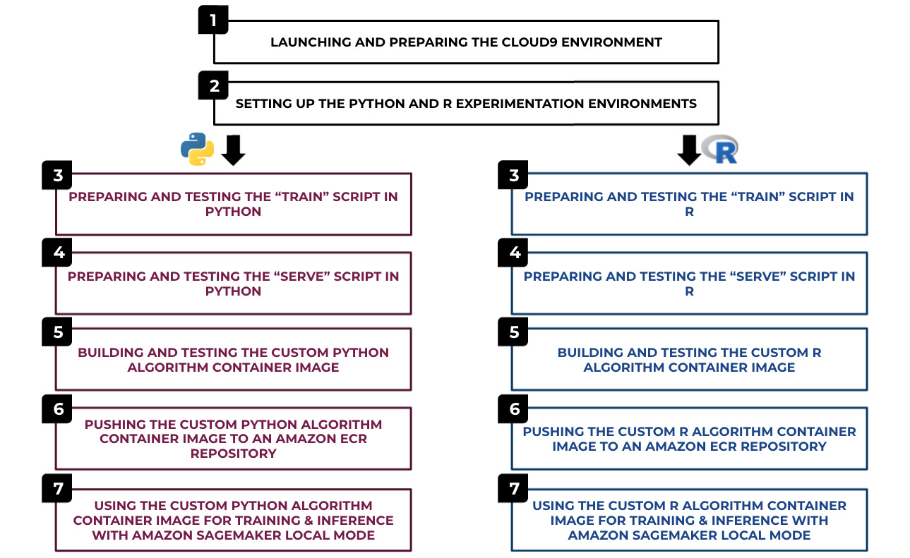
Figure 2.1 – Chapter 2 recipes

In this chapter, we will work on creating and using our own algorithm container images in Amazon SageMaker. With this approach, we can use any custom scripts, libraries, frameworks, or algorithms. This chapter will enlighten us on how we can make the most out of Amazon SageMaker through custom container images. As shown in the preceding diagram, we will start by setting up a cloud-based integrated development environment with AWS Cloud9, where we will prepare, configure, and test the scripts before building the container image. Once we have the environment ready, we will code the train and serve scripts inside this environment. The train script will be used during training, while the serve script will be used for the inference endpoint of the deployed model. We will then prepare a Dockerfile that makes use of the train and serve scripts that we generated in the earlier steps. Once this Dockerfile is ready, we will build the custom container image and use the container image for training and inference with the SageMaker Python SDK. We will work on these steps in both Python and R.

We will cover the following recipes in this chapter:

• Launching and preparing the Cloud9 environment
• Setting up the Python and R experimentation environments
• Preparing and testing the train script in Python
• Preparing and testing the serve script in Python
• Building and testing the custom Python algorithm container image
• Pushing the custom Python algorithm container image to an Amazon ECR repository
• Using the custom Python algorithm container image for training and inference with Amazon SageMaker Local Mode
• Preparing and testing the train script in R
• Preparing and testing the serve script in R
• Building and testing the custom R algorithm container image
• Pushing the custom R algorithm container image to an Amazon ECR repository
• Using the custom R algorithm container image for training and inference with Amazon SageMaker Local Mode

After we have completed the recipes in this chapter, we will be ready to use our own algorithms and custom container images in SageMaker. This will significantly expand what we can do outside of the built-in algorithms and container images provided by SageMaker. At the same time, the techniques and concepts used in this chapter will give you the exposure and experience needed to handle similar requirements, as you will see in the upcoming chapters.

You will need the following to complete the recipes in this chapter:

• A running Amazon SageMaker notebook instance (for example, ml.t2.large). Feel free to use the SageMaker notebook instance we launched in the Launching an Amazon SageMaker Notebook instance recipe of Chapter 1, Getting Started with Machine Learning Using Amazon SageMaker.
• Permission to manage the Amazon SageMaker, Amazon S3, and AWS Cloud9 resources if you're using an AWS IAM user with a custom URL. It is recommended to be signed in as an AWS IAM user instead of using the root account in most cases. For more information, feel free to take a look at https://docs.aws.amazon.com/IAM/latest/UserGuide/best-practices.html.

The Jupyter Notebooks, source code, and CSV files used for each chapter are available in this book's GitHub repository: https://github.com/PacktPublishing/Machine-Learning-with-Amazon-SageMaker-Cookbook/tree/master/Chapter02.

Check out the following link to see the relevant Code in Action video:

https://bit.ly/38Uvemc

In this recipe, we will launch and configure an AWS Cloud9 instance running an Ubuntu server. This will serve as the experimentation and simulation environment for the other recipes in this chapter. After that, we will resize the volume attached to the instance so that we can build container images later. This will ensure that we don't have to worry about disk space issues while we are working with Docker containers and container images. In the succeeding recipes, we will be preparing the expected file and directory structure that our train and serve scripts will expect when they are inside the custom container.

Important note

Why go through all this effort of preparing an experimentation environment? Once we have finished preparing the experimentation environment, we will be able to prepare, test, and update the custom scripts quickly, without having to use the fit() and deploy() functions from the SageMaker Python SDK during the initial stages of writing the script. With this approach, the feedback loop is much faster, and we will detect the issues in our script and container image before we even attempt using these with the SageMaker Python SDK during training and deployment.

Getting ready

Make sure you have permission to manage the AWS Cloud9 and EC2 resources if you're using an AWS IAM user with a custom URL. It is recommended to be signed in as an AWS IAM user instead of using the root account in most cases.

How to do it…

The steps in this recipe can be divided into three parts:

• Launching a Cloud9 environment
• Increasing the disk space of the environment
• Making sure that the volume configuration changes get reflected by rebooting the instance associated with the Cloud9 environment

We'll begin by launching the Cloud9 environment with the help of the following steps:

1. Click Services on the navigation bar. A list of services will be shown in the menu. Under Developer Tools, look for Cloud9 and then click the link to navigate to the Cloud9 console:
   

   Figure 2.2 – Looking for the AWS Cloud9 service under Developer Tools

   In the preceding screenshot, we can see the services after clicking the Services link on the navigation bar.

2. In the Cloud9 console, navigate to Your environments using the sidebar and click Create environment:
   

   Figure 2.3 – Create environment button

   Here, we can see that the Create environment button is located near the top-right corner of the page.

3. Specify the environment's name (for example, Cookbook Experimentation Environment) and, optionally, a description for your environment. Click Next step afterward:
   

   Figure 2.4 – Name environment form

   Here, we have the Name environment form, where we can specify the name and description of our Cloud9 environment.

4. Select the Create a new EC2 instance for environment (direct access) option under Environment type, t3.small under Instance type, and Ubuntu Server 18.04 LTS under Platform:
   

   Figure 2.5 – Environment settings

   We can see the different configuration settings here. Feel free to choose a different instance type as needed.

5. Under Cost-saving setting, select After one hour. Leave the other settings as-is and click Next step:
   

   Figure 2.6 – Other configuration settings

   Here, we can see that we have selected a Cost-saving setting of After one hour. This means that after an hour of inactivity, the EC2 instance linked to the Cloud9 environment will be automatically turned off to save costs.

6. Review the configuration you selected in the previous steps and then click Create environment:
   

   Figure 2.7 – Create environment button

   After clicking the Create environment button, it may take a minute or so for the environment to be ready. Once the environment is ready, check the different sections of the IDE:

   

   Figure 2.8 – AWS Cloud9 development environment

   As you can see, we have the file tree on the left-hand side. At the bottom part of the screen, we have the Terminal, where we can run our Bash commands. The largest portion, at the center of the screen, is the Editor, where we can edit the files.

   Now, we need to increase the disk space.

7. Using the Terminal at the bottom section of the IDE, run the following command:

   lsblk

   With the lsblk command, we will get information about the available block devices, as shown in the following screenshot:

   

   Figure 2.9 – Result of the lsblk command

   Here, we can see the results of the lsblk command. At this point, the root volume only has 10G of disk space (minus what is already in the volume).

8. At the top left section of the screen, click AWS Cloud9. From the dropdown list, click Go To Your Dashboard:
   

   Figure 2.10 – How to go back to the AWS Cloud9 dashboard

   This will open a new tab showing the Cloud9 dashboard.

9. Navigate to the EC2 console using the search bar. Type ec2 in the search bar and click the EC2 service from the list of results:
   

   Figure 2.11 – Using the search bar to navigate to the EC2 console

   Here, we can see that the search bar quickly gives us a list of search results after we have typed in ec2.

10. In the EC2 console, click Instances (running) under Resources:
    

    Figure 2.12 – Instances (running) link under Resources

    We should see the link we need to click under the Resources pane, as shown in the preceding screenshot.

11. Select the EC2 instance corresponding to the Cloud9 environment we launched in the previous set of steps. It should contain aws-cloud9 and the name we specified while creating the environment. In the bottom pane showing the details, click the Storage tab to show Root device details and Block devices.
12. Inside the Storage tab, scroll down to the bottom of the page to locate the volumes under Block devices:
    

    Figure 2.13 – Storage tab

    Here, we can see the Storage tab showing Root device details and Block devices.

13. You should see an attached volume with 10 GiB for the volume size. Click the link under Volume ID (for example, vol-0130f00a6cf349ab37). Take note that this Volume ID will be different for your volume:
    

    Figure 2.14 – Looking for the volume attached to the EC2 instance

    You will be redirected to the Elastic Block Store Volumes page, which shows the details of the volume attached to your instance:

    

    Figure 2.15 – Elastic Block Store Volumes page

    Here, we can see that the size of the volume is currently set to 10 GiB.

14. Click Actions and then Modify Volume:
    

    Figure 2.16 – Modify Volume

    This is where we can find the Modify Volume option.

15. Set Size to 100 and click Modify:
    

    Figure 2.17 – Modifying the volume

    As you can see, we specified a new volume size of 100 GiB. This should be more than enough to help us get through this chapter and build our custom algorithm container image.

16. Click Yes to confirm the volume modification action:
    

    Figure 2.18 – Modify Volume confirmation dialog

    We should see a confirmation screen here after clicking Modify in the previous step.

17. Click Close upon seeing the confirmation dialog:
    

    Figure 2.19 – Modify Volume Request Succeeded message

    Here, we can see a message stating Modify Volume Request Succeeded. At this point, the volume modification is still pending and we need to wait about 10-15 minutes for this to complete. Feel free to check out the How it works… section for this recipe while waiting.

18. Click the refresh button (the two rotating arrows) so that the volume state will change to the correct state accordingly:
    

    Figure 2.20 – Refresh button

    Clicking the refresh button will update State from in-use (green) to in-use – optimizing (yellow):

    

    Figure 2.21 – In-use state – optimizing (yellow)

    Here, we can see that the volume modification step has not been completed yet.

19. After a few minutes, State of the volume will go back to in-use (green):
    

    Figure 2.22 – In-use state (green)

    When we see what is shown in the preceding screenshot, we should celebrate as this means that the volume modification step has been completed!

    Now that the volume modification step has been completed, our next goal is to make sure that this change is reflected in our environment.

20. Navigate back to the browser tab of the AWS Cloud9 IDE. In the Terminal, run lsblk:

    lsblk

    Running lsblk should yield the following output:

    

    Figure 2.23 – Partition not yet reflecting the size of the root volume

    As you can see, while the size of the root volume, /dev/nvme0n1, reflects the new size, 100G, the size of the /dev/nvme0n1p1 partition reflects the original size, 10G.

    There are multiple ways to grow the partition, but we will proceed by simply rebooting the EC2 instance so that the size of the /dev/nvme0n1p1 partition will reflect the size of the root volume, which is 100G.

21. Navigate back to the EC2 Volumes page and select the EC2 volume attached to the Cloud9 instance. At the bottom portion of the screen showing the volume's details, locate the Attachment information value under the Description tab. Click the Attachment information link:
    

    Figure 2.24 – Attachment information

    Clicking this link will redirect us to the EC2 Instances page. It will automatically select the EC2 instance of our Cloud9 environment:

    

    Figure 2.25 – EC2 instance of the Cloud9 environment

    The preceding screenshot shows the EC2 instance linked to our Cloud9 environment.

22. Click Instance state at the top right of the screen and click Reboot instance:
    

    Figure 2.26 – Reboot instance

    This is where we can find the Reboot instance option.

23. Navigate back to the browser tab showing the AWS Cloud9 environment IDE. It should take a minute or two to complete the reboot step:
    

    Figure 2.27 – Instance is still rebooting

    We should see a screen similar to the preceding one.

24. Once connected, run lsblk in the Terminal:

    lsblk

    We should get a set of results similar to what is shown in the following screenshot:

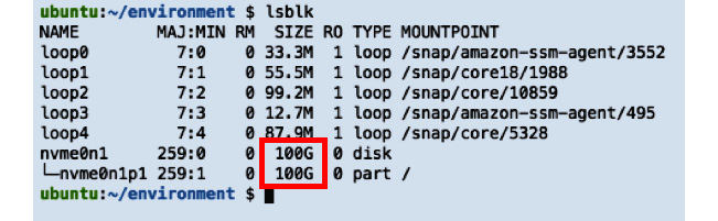
Figure 2.28 – Partition now reflecting the size of the root instance

As we can see, the /dev/nvme0n1p1 partition now reflects the size of the root volume, which is 100G.

That was a lot of setup work, but this will be definitely worth it, as you will see in the next few recipes in this chapter. Now, let's see how this works!

How it works…

In this recipe, we launched a Cloud9 environment where we will prepare the custom container image. When building Docker container images, it is important to note that each container image consumes a bit of disk space. This is why we had to go through a couple of steps to increase the volume attached to the EC2 instance of our Cloud9 environment. This recipe was composed of three parts: launching a new Cloud9 environment, modifying the mounted volume, and rebooting the instance.

Launching a new Cloud9 environment involves using a CloudFormation template behind the scenes. This CloudFormation template is used as the blueprint when creating the EC2 instance:

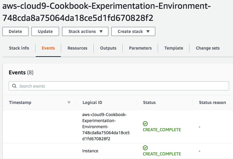
Figure 2.29 – CloudFormation stack

Here, we have a CloudFormation stack that was successfully created. What's CloudFormation? AWS CloudFormation is a service that helps developers and DevOps professionals manage resources using templates written in JSON or YAML. These templates get converted into AWS resources using the CloudFormation service.

At this point, the EC2 instance should be running already and we can use the Cloud9 environment as well:

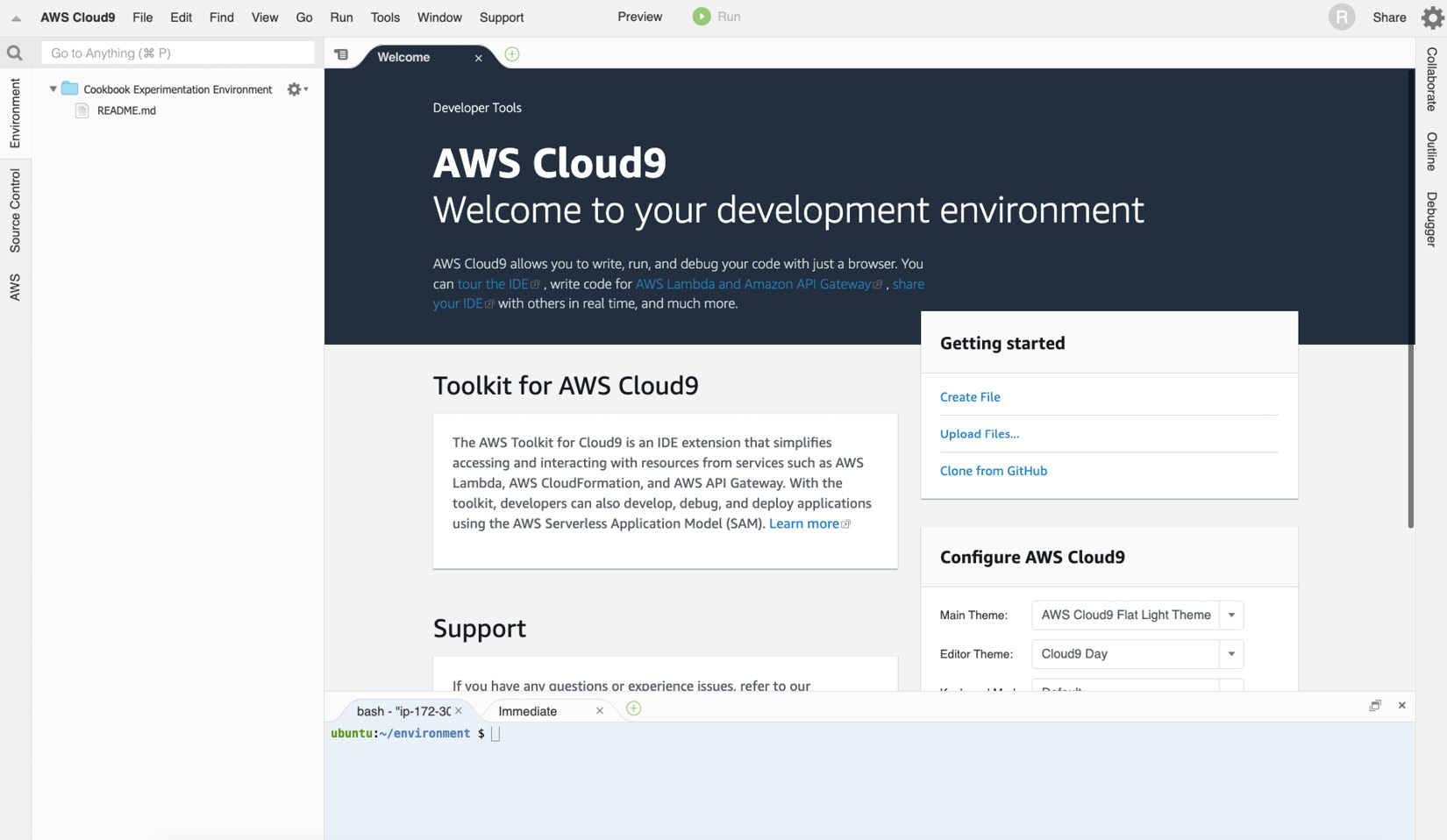
Figure 2.30 – AWS Cloud9 environment

We should be able to see the preceding output once the Cloud9 environment is ready. If we were to use the environment right away, we would run into disk space issues as we will be working with Docker images, which take up a bit of space. To prevent these issues from happening later on, we modified the volume in this recipe and restarted the EC2 instance so that this volume modification gets reflected right away.

Important note

In this recipe, we took a shortcut and simply restarted the EC2 instance. If we were running a production environment, we should avoid having to reboot and follow this guide instead: https://docs.aws.amazon.com/AWSEC2/latest/UserGuide/recognize-expanded-volume-linux.html.

Note that we can also use a SageMaker Notebook instance that's been configured with root access enabled as a potential experimentation environment for our custom scripts and container images, before using them in SageMaker. The issue here is that when using a SageMaker Notebook instance, it reverts to how it was originally configured every time we turn off and reboot the instance. This makes us lose certain directories and installed packages, which is not ideal.

In the previous recipe, we launched a Cloud9 environment. In this recipe, we will be preparing the expected file and directory structure inside this environment. This will help us prepare and test our train and serve scripts before running them inside containers and before using these with the SageMaker Python SDK:

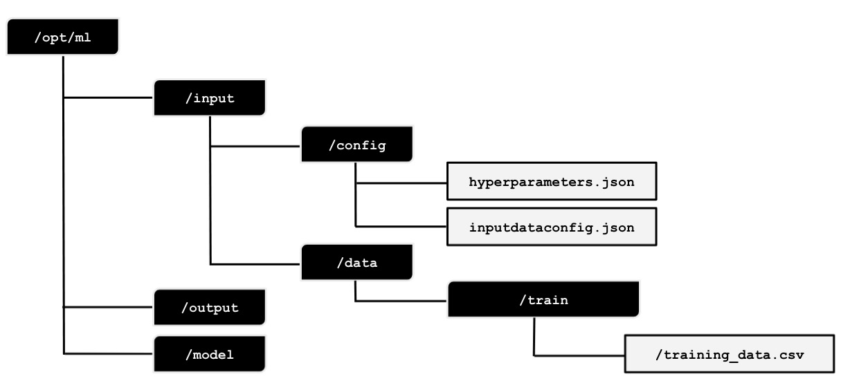
Figure 2.31 – Expected file and directory structure inside /opt/ml

We can see the expected directory structure in the preceding diagram. We will prepare the expected directory structure inside /opt/ml. After that, we will prepare the hyperparameters.json, inputdataconfig.json, and training_data.csv files. In the succeeding recipes, we will use these files when preparing and testing the train and serve scripts.

Getting ready

Here are the prerequisites for this recipe:

• This recipe continues from Launching and preparing the Cloud9 environment.
• We will need the S3 bucket from the Preparing the Amazon S3 bucket and the training dataset for the linear regression experiment recipe of Chapter 1. We will also need the training_data.csv file inside this S3 bucket. After performing the train-test split, we uploaded the CSV file to the S3 bucket in the Training your first model in Python recipe of Chapter 1. If you skipped this recipe, you can upload the training_data.csv file from this book's GitHub repository (https://github.com/PacktPublishing/Machine-Learning-with-Amazon-SageMaker-Cookbook) to the S3 bucket instead.

How to do it…

In the first set of steps in this recipe, we will use the Terminal to run the commands. We will continue where we left off in the previous Launching and preparing the Cloud9 environment recipe:

1. Use the pwd command to see the current working directory:

   pwd

2. Navigate to the /opt directory:

   cd /opt

3. Create the /opt/ml directory using the mkdir command. Make sure that you are inside the /opt directory before running the sudo mkdir ml command. Modify the ownership configuration of the /opt/ml directory using the chown command. This will allow us to manage the contents of this directory without using sudo over and over again in the succeeding steps:

   sudo mkdir -p ml
   sudo chown ubuntu:ubuntu ml

4. Navigate to the ml directory using the cd Bash command. Run the following commands to prepare the expected directory structure inside the /opt/ml directory. Make sure that you are inside the ml directory before running these commands. The -p flag will automatically create the required parent directories first, especially if some of the directories in the specified path do not exist yet. In this case, if the input directory does not exist, the mkdir -p input/config command will create it first before creating the config directory inside it:

   cd ml
   mkdir -p input/config
   mkdir -p input/data/train
   mkdir -p output/failure
   mkdir -p model

   As we will see later, these directories will contain the files and configuration data that we'll pass as parameter values when we initialize the Estimator.

   Important note

   Again, if you are wondering why we are creating these directories, the answer is that we are preparing an environment where we can test and iteratively build our custom scripts first, before using the SageMaker Python SDK and API. It is hard to know if a script is working unless we run it inside an environment that has a similar set of directories and files. If we skip this step and use the custom training script directly with the SageMaker Python SDK, we will spend a lot of time debugging potential issues as we have to wait for the entire training process to complete (at least 5-10 minutes), before being able to fix a scripting bug and try again to see if the fix worked. With this simulation environment in place, we will be able to test our custom script and get results within a few seconds instead. As you can see, we can iterate rapidly if we have a simulation environment in place.

   The following is the expected directory structure:

   

   Figure 2.32 – Expected file and folder structure after running the mkdir commands

   Here, we can see that there are /config and /data directories inside the /input directory. The /config directory will contain the hyperparameters.json file and the inputdataconfig.json file, as we will see later. We will not be using the /output directory in the recipes in this chapter, but this is where we can create a file called failure in case the training job fails. The failure file should describe why the training job failed to help us debug and adjust it in case the failure scenario happens.

5. Install and use the tree command:

   sudo apt install tree
   tree

   We should get a tree structure similar to the following:

   

   Figure 2.33 – Result of the tree command

   Here, we can see the expected directory structure.

6. Create the /home/ubuntu/environment/opt directory using mkdir and create two directories inside it called ml-python and ml-r:

   mkdir -p /home/ubuntu/environment/opt
   cd /home/ubuntu/environment/opt
   mkdir -p ml-python ml-r

7. Create a soft symbolic link to make it easier to manage the files and directories using the AWS Cloud9 interface:

   sudo ln -s /opt/ml  /home/ubuntu/environment/opt/ml

   Given that we are performing this step inside a Cloud9 environment, we will be able to easily create and modify the files using the visual editor, instead of using vim or nano in the command line. What this means is that changes that are made inside the /home/ubuntu/environment/opt/ml directory will also be reflected inside the /opt/ml directory. This will allow us to use a visual editor to easily create and modify files:

   

   Figure 2.34 – File tree showing the symlinked /opt/ml directory

   We should see the directories inside the /opt/ml directory in the file tree, as shown in the preceding screenshot.

   The next set of steps focus on adding the dummy files to the experimentation environment.

8. Using the file tree, navigate to the /opt/ml/input/config directory. Right-click on the config directory and select New File:
   

   Figure 2.35 – Creating a new file inside the config directory

9. Name the new file hyperparameters.json. Double-click the new file to open it in the Editor pane:
   

   Figure 2.36 – Empty hyperparameters.json file

   Here, we have an empty hyperparameters.json file inside the /opt/ml/input/config directory.

10. Set the content of the hyperparameters.json file to the following line of code:

    {"a": 1, "b": 2}

    Your Cloud9 environment IDE's file tree and Editor pane should look as follows:

    

    Figure 2.37 – Specifying a sample JSON value to the hyperparameters.json file

    Make sure to save it by clicking the File menu and then clicking Save. You can also use Cmd + S or Ctrl + S to save the file, depending on the operating system you are using.

11. In a similar fashion, create a new file called inputdataconfig.json inside /opt/ml/input/config. Open the inputdataconfig.json file in the Editor pane and set its content to the following line of code:

    {"train": {"ContentType": "text/csv", "RecordWrapperType": "None", "S3DistributionType": "FullyReplicated", "TrainingInputMode": "File"}}

    Your Cloud9 environment IDE's file tree and Editor pane should look as follows:

    

    Figure 2.38 – The inputdataconfig.json file

    In the next set of steps, we will download the training_data.csv file from Chapter 1, Getting Started with Machine Learning Using Amazon SageMaker, to the experimentation environment. In the Training your first model in Python recipe from Chapter 1, Getting Started with Machine Learning Using Amazon SageMaker, we uploaded a training_data.csv file to an Amazon S3 bucket:

    

    Figure 2.39 – The training_data.csv file inside the S3 bucket

    In case you skipped these recipes in Chapter 1, make sure that you check out this book's GitHub repository (https://github.com/PacktPublishing/Machine-Learning-with-Amazon-SageMaker-Cookbook) and upload the training_data.csv file to the S3 bucket. Note that the recipes in this chapter assume that the training_data.csv file is inside s3://S3_BUCKET/PREFIX/input, where S3_BUCKET is the name of the S3 bucket and PREFIX is the folder's name. If you have not created an S3 bucket yet, follow the steps in the Preparing the Amazon S3 bucket and the training dataset for the linear regression experiment recipe of Chapter 1 as we will need this S3 bucket for all the chapters in this book.

12. In the Terminal of the Cloud9 IDE, run the following commands to download the training_data.csv file from S3 to the /opt/ml/input/data/train directory:

    cd /opt/ml/input/data/train
    S3_BUCKET="<insert bucket name here>"
    PREFIX="chapter01"
    aws s3 cp s3://$S3_BUCKET/$PREFIX/input/training_data.csv training_data.csv

    Make sure that you set the S3_BUCKET value to the name of the S3 bucket you created in the Preparing the Amazon S3 bucket and the training dataset for the linear regression experiment recipe of Chapter 1.

13. In the file tree, double-click the training_data.csv file inside the /opt/ml/input/data/train directory to open it in the Editor pane:
    

    Figure 2.40 – The training_data.csv file inside the experimentation environment

    As shown in the preceding screenshot, the training_data.csv file contains the y values in the first column and the x values in the second column.

    In the next set couple of steps, we will install a few prerequisites in the Terminal.

14. In the Terminal, run the following scripts to make the R recipes work in the second half of this chapter:

    sudo apt-get -y update
    sudo apt-get install -y --no-install-recommends wget
    sudo apt-get install -y --no-install-recommends r-base
    sudo apt-get install -y --no-install-recommends r-base-dev
    sudo apt-get install -y --no-install-recommends ca-certificates

15. Install the command-line JSON processor; that is, jq:

    sudo apt install -y jq

    In the last set of steps in this recipe, we will create the files inside the ml-python and ml-r directories. In the Building and testing the custom Python algorithm container image and Building and testing the custom R algorithm container image recipes, we will copy these files inside the container while building the container image with the docker build command.

16. Right-click on the ml-python directory and then click New File from the menu to create a new file, as shown here. Name the new file train:
    

    Figure 2.41 – Creating a new file inside the ml-python directory

    Perform this step two more times so that there are three files inside the ml-python directory called train, serve, and Dockerfile. Take note that these files are empty for now:

    

    Figure 2.42 – Files inside the ml-python directory

    The preceding screenshot shows these three empty files. We will work with these later in the Python recipes in this chapter.

17. Similarly, create four new files inside the ml-r directory called train, serve, api.r, and Dockerfile:

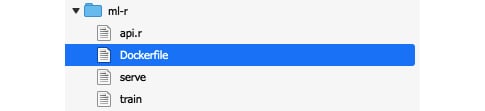
Figure 2.43 – Files inside the ml-r directory

The preceding screenshot shows these four empty files. We will be working with these later in the R recipes in this chapter.

Let's see how this works!

How it works…

In this recipe, we prepared the experimentation environment where we will iteratively build the train and serve scripts. Preparing the train and serve scripts is an iterative process. We will need an experimentation environment to ensure that the scripts work before using them inside a running container. Without the expected directory structure and the dummy files, it would be hard to test and develop the train and serve scripts in a way that seamlessly translates to using these with SageMaker.

Let's discuss and quickly describe how the train script should work. The train script may load one or more of the following:

• hyperparameters.json: Contains the hyperparameter configuration data set in Estimator
• inputdataconfig.json: Contains the information where the training dataset is stored
• <directory>/<data file>: Contains the training dataset's input (for example, train/training.csv)

We will have a closer look at preparing and testing train scripts in the Preparing and testing the train script in Python and Preparing and testing the train script in R recipes in this chapter.

Now, let's talk about the serve script. The serve script expects the model file(s) inside the /opt/ml/model directory. Take note that one or more of these files may not exist, and this depends on the configuration parameters and arguments we have set using the SageMaker Python SDK. This also depends on what we write our script to need. We will have a closer look at preparing and testing serve scripts in the Preparing and testing the serve script in Python and Preparing and testing the serve script in R recipes later in this chapter.

There's more…

As we are about to work on the recipes specific to Python and R, we need to have a high-level idea of how these all fit together. In the succeeding recipes, we will build a custom container image containing the train and serve scripts. This container image will be used during training and deployment using the SageMaker Python SDK. In this section, we will briefly discuss what happens under the hood when we run the fit() function while using a custom container image. I believe it would be instructive to reiterate here that we built those directories and dummy files to create the train and serve scripts that the fit() and deploy() commands will run.

If you are wondering what the train and serve script files are for, these script files are executed inside a container behind the scenes by SageMaker when the fit() and deploy() functions from the SageMaker Python SDK are used. We will write and test these scripts later in this chapter. When we use the fit() function, SageMaker starts the training job. Behind the scenes, SageMaker performs the following set of steps:

Preparation and configuration

1. One or more ML instances are launched. The number and types of ML instances for the training job depend on the instance_count and instance_type arguments specified when initializing the Estimator class:

   container="<insert image uri of the custom container image>"
   estimator = sagemaker.estimator.Estimator(
       container,
       instance_count=1, 
       instance_type='local',
       ...
   )
   estimator.fit({'train': train})

2. The hyperparameters specified using the set_hyperparameters() function are copied and stored as a JSON file called hyperparameters.json inside the /opt/ml/input/config directory. Take note that our custom container will not have this file at the start, and that SageMaker will create this file for us automatically when the training job starts.

Training

1. The input data we have specified in the fit() function will be loaded by SageMaker (for example, from the specified S3 bucket) and copied into /opt/ml/input/data/. For each of the input data channels, a directory containing the relevant files will be created inside the /opt/ml/input/data directory. For example, if we used the following line of code using the SageMaker Python SDK, then we would expect the /opt/ml/input/data/apple and /opt/ml/data/banana directories when the train script starts to run:

   estimator.fit({'apple': TrainingInput(...),'banana': TrainingInput(...)})

2. Next, your custom train script runs. It loads the configuration files, hyperparameters, and the data files from the directories inside /opt/ml. It then trains a model using the training dataset and, optionally, a validation dataset. The model is then serialized and stored inside the /opt/ml/model directory.

   Note

   Do not worry if you have no idea how the train script looks like as we will discuss the train script in detail later, in the succeeding recipes.

3. SageMaker expects the model output file(s) inside the /opt/ml/model directory. After the training script has finished executing, SageMaker automatically copies the contents of the /opt/ml/model directory and stores it inside the target S3 bucket and path (inside model.tar.gz). Take note that we can specify the target S3 bucket and path by setting the output_path argument when initializing Estimator with the SageMaker Python SDK.
4. If there is an error running the script, SageMaker will look for a failure file inside the /opt/ml/output directory. If it exists, the text output stored in this file will be loaded when the DescribeTrainingJob API is used.
5. The created ML instances are deleted. The billable time is returned to the user.

Deployment

When we use the deploy() function, SageMaker starts the model deployment step. The assumption when running the deploy() function is that the model.tar.gz file is stored inside the target S3 bucket path.

1. One or more ML instances are launched. The number and types of ML instances for the deployment step depend on the instance_count and instance_type arguments specified when using the deploy() function:

   predictor = estimator.deploy(
       initial_instance_count=1, 
       instance_type='local', 
       endpoint_name="custom-local-py-endpoint")

2. The model.tar.gz file is copied from the S3 bucket and the files are extracted inside the /opt/ml/model directory.
3. Next, your custom serve script runs. It uses the model files inside the /opt/ml/model directory to deserialize and load the model. The serve script then runs an API web server with the required /ping and /invocations endpoints.

Inference

1. After deployment, the predict() function calls the /invocations endpoint to use the loaded model for inference.

This should give us a better idea and understanding of the purpose of the files and directories we have prepared in this recipe. If you are a bit overwhelmed by the level of detail in this section, do not worry as things will become clearer as we work on the next few recipes in this chapter!

In this recipe, we will write a train script in Python that allows us to train a linear model with scikit-learn. Here, we can see that the train script inside a running custom container makes use of the hyperparameters, input data, and the configuration specified in the Estimator instance using the SageMaker Python SDK:

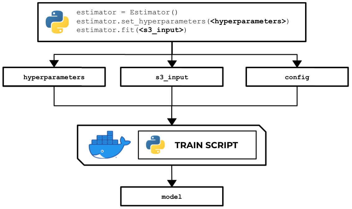
Figure 2.44 – How the train script is used to produce a model

There are several options when running a training job – use a built-in algorithm, use a custom train script and custom Docker container images, or use a custom train script and prebuilt Docker images. In this recipe, we will focus on the second option, where we will prepare and test a bare minimum training script in Python that builds a linear model for a specific regression problem.

Once we have finished working on this recipe, we will have a better understanding of how SageMaker works behind the scenes. We will see where and how to load and use the configuration and arguments we have specified in the SageMaker Python SDK Estimator.

Getting ready

Make sure you have completed the Setting up the Python and R experimentation environments recipe.

How to do it…

The first set of steps in this recipe focus on preparing the train script. Let's get started:

1. Inside the ml-python directory, double-click the train file to open the file inside the Editor pane:
   

   Figure 2.45 – Empty ml-python/train file

   Here, we have an empty train file. In the lower right-hand corner of the Editor pane, you can change the syntax highlight settings to Python.

2. Add the following lines of code to start the train script to import the required packages and libraries:

   #!/usr/bin/env python3
   import json
   import pprint
   import pandas as pd
   from sklearn.linear_model import LinearRegression
   from joblib import dump, load
   from os import listdir

   In the preceding block of code, we imported the following:

   • json for utility functions when working with JSON data
   • pprint to help us "pretty-print" nested structures such as dictionaries
   • pandas to help us read CSV files and work with DataFrames
   • LinearRegression from the sklearn library for training a linear model when we run the train script
   • joblib for saving and loading a model
   • listdir from the os module to help us list the files inside a directory
3. Define the PATHS constant and the get_path() function. The get_path() function will be handy in helping us manage the paths and locations of the primary files and directories used in the script:

   PATHS = {
       'hyperparameters': 'input/config/hyperparameters.json',
       'input': 'input/config/inputdataconfig.json',
       'data': 'input/data/',
       'model': 'model/'
   }
       
   def get_path(key):
       return '/opt/ml/' + PATHS[key]

   If we want to get the path of the hyperparameters.json file, we can use get_path("hyperparameters") instead of using the absolute path in our code.

   Important note

   In this chapter, we will intentionally use get_path for the function name. If you have been using Python for a while, you will probably notice that this is definitely not Pythonic code! Our goal is for us to easily find the similarities and differences between the Python and R scripts, so we made the function names the same for the most part.

4. Next, add the following lines just after the get_path() function definition from the previous step. These additional functions will help us later once we need to load and print the contents of the JSON files we'll be working with (for example, hyperparameters.json):

   def load_json(target_file):
       output = None
       
       with open(target_file) as json_data:
           output = json.load(json_data)
       
       return output
       
   def print_json(target_json):
       pprint.pprint(target_json, indent=4)

5. Include the following functions as well in the train script (after the print_json() function definition):

   def inspect_hyperparameters():
       print('[inspect_hyperparameters]')
       hyperparameters_json_path = get_path(
           'hyperparameters'
       )
       print(hyperparameters_json_path)
       
       hyperparameters = load_json(
           hyperparameters_json_path
       )
       print_json(hyperparameters)
       
   def list_dir_contents(target_path):
       print('[list_dir_contents]')
       output = listdir(target_path)
       print(output)
       
       return output

   The inspect_hyperparameters() function allows us to inspect the contents of the hyperparameters.json file inside the /opt/ml/input/config directory. The list_dir_contents() function, on the other hand, allows us to display the contents of a target directory. We will use this later to check the contents of the training input directory.

6. After that, define the inspect_input() function. This allows us to inspect the contents of inputdataconfig.json inside the /opt/ml/input/config directory:

   def inspect_input():
       print('[inspect_input]')
       input_config_json_path = get_path('input')
       print(input_config_json_path)
       input_config = load_json(input_config_json_path)
       print_json(input_config)

7. Define the load_training_data() function. This function accepts a string value pointing to the input data directory and returns the contents of a CSV file inside that directory:

   def load_training_data(input_data_dir):
       print('[load_training_data]')    
       files = list_dir_contents(input_data_dir)
       training_data_path = input_data_dir + files[0]
       print(training_data_path)
       
       df = pd.read_csv(
           training_data_path, header=None
       )
       print(df)
       
       y_train = df[0].values
       X_train = df[1].values
       return (X_train, y_train)

   The flow inside the load_training_data() function can be divided into two parts – getting the specific path of the CSV file containing the training data, and then reading the contents of the CSV file using the pd.read_csv() function and returning the results inside a tuple of lists.

   Note

   Of course, the load_training_data() function we've implemented here assumes that there is only one CSV file inside that directory, so feel free to modify the following implementation when you are working with more than one CSV file inside the provided directory. At the same time, this function implementation only supports CSV files, so make sure to adjust the code block if you need to support multiple input file types.

8. Define the get_input_data_dir() function:

   def get_input_data_dir():
       print('[get_input_data_dir]')
       key = 'train'
       input_data_dir = get_path('data') + key + '/'
       return input_data_dir

9. Define the train_model() function:

   def train_model(X_train, y_train):
       print('[train_model]')
       model = LinearRegression()
       model.fit(X_train.reshape(-1, 1), y_train)
       return model

10. Define the save_model() function:

    def save_model(model):
        print('[save_model]')
        filename = get_path('model') + 'model'
        print(filename)
        dump(model, filename)
        print('Model Saved!')

11. Create the main() function, which executes the functions we created in the previous steps:

    def main():
        inspect_hyperparameters()
        inspect_input()
        input_data_dir = get_input_data_dir()
        X_train, y_train = load_training_data(
            input_data_dir
        )
        model = train_model(X_train, y_train)
        save_model(model)

    This function simply inspects the hyperparameters and input configuration, trains a linear model using the data loaded from the input data directory, and saves the model using the save_model() function.

12. Finally, run the main() function:

    if __name__ == "__main__":
        main()

    The __name__ variable is set to "__main__" when the script is executed as the main program. This if condition simply tells the script to run if we're using it as the main program. If this script is being imported by another script, then the main() function will not run.

    Tip

    You can access a working copy of the train script file in the Machine Learning with Amazon SageMaker Cookbook GitHub repository: https://github.com/PacktPublishing/Machine-Learning-with-Amazon-SageMaker-Cookbook/blob/master/Chapter02/ml-python/train.

    Now that we are done with the train script, we will use the Terminal to perform the last set of steps in this recipe.

    The last set of steps focus on installing a few script prerequisites:

13. Open a new Terminal:
    

    Figure 2.46 – New Terminal

    Here, we can see how to create a new Terminal tab. We simply click the plus (+) button and then choose New Terminal.

14. In the Terminal at the bottom pane, run python3 --version:

    python3 --version

    Running this line of code should return a similar set of results to what is shown in the following screenshot:

    

    Figure 2.47 – Result of running python3 --version in the Terminal

    Here, we can see that our environment is using Python version 3.6.9.

15. Install pandas using pip. The pandas library is used when working with DataFrames (tables):

    pip3 install pandas

16. Install sklearn using pip. The scikit-learn library is a machine learning library that features several algorithms for classification, regression, and clustering problems:

    pip3 install sklearn

17. Navigate to the ml-python directory:

    cd /home/ubuntu/environment/opt/ml-python

18. To make the train script executable, run the following command in the Terminal:

    chmod +x train

19. Test the train script in your AWS Cloud9 environment by running the following command in the Terminal:

    ./train

    Running the previous lines of code will yield results similar to the following:

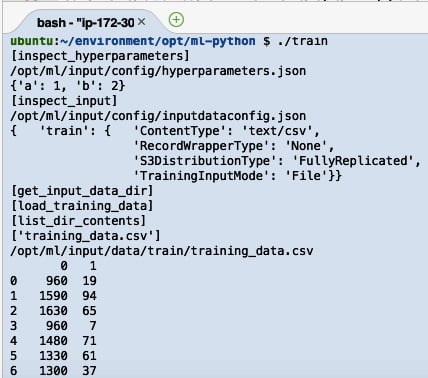
Figure 2.48 – Result of running the train script

Here, we can see the logs that were produced by the train script. After the train script has been successfully executed, we expect the model files to be stored inside the /opt/ml/model directory.

Now, let's see how this works!

How it works…

In this recipe, we prepared a custom train script using Python. The script starts by identifying the input paths and loading the important files to help set the context of the execution. This train script demonstrates how the input and output values are passed around between the SageMaker Python SDK (or API) and the custom container. It also shows how to load the training data, train a model, and save a model.

When the Estimator object is initialized and configured, some of the specified values, including the hyperparameters, are converted from a Python dictionary into JSON format in an API call when invoking the fit() function. The API call on the SageMaker platform then proceeds to create and mount the JSON file inside the environment where the train script is running. It works the same way as it does with the other files loaded by the train script file, such as the inputdataconfig.json file.

If you are wondering what is inside the inputdataconfig.json file, refer to the following code block for an example of what it looks like:

{"<channel name>": {"ContentType": "text/csv", 
       "RecordWrapperType": "None",
       "S3DistributionType": "FullyReplicated",
       "TrainingInputMode": "File"}} 

For each of the input channels, a corresponding set of properties is specified in this file. The following are some of the common properties and values that are used in this file. Of course, the values here depend on the type of data and the algorithm being used in the experiment:

• ContentType – Valid Values: text/csv, image/jpeg, application/x-recordio-protobuf, and more.
• RecordWrapperType – Valid Values: None or RecordIO. The RecordIO value is set only when the TrainingInputMode value is set to Pipe. The training algorithm requires the RecordIO format for the input data, and the input data is not in RecordIO format yet.
• S3DistributionType – Valid Values: FullyReplicated or ShardedByS3Key. If the value is set to FullyReplicated, the entire dataset is copied on each ML instance that's launched during model training. On the other hand, when the value is set to ShardedByS3Key, each machine that's launched and used during model training makes use of a subset of the training data provided.
• TrainingInputMode – Valid Values: File or Pipe. When the File input mode is used, the entire dataset is downloaded first before the training job starts. On the other hand, the Pipe input mode is used to speed up training jobs, start faster, and requires less disk space. This is very useful when dealing with large datasets. If you are planning to support the Pipe input mode in your custom container, the directories inside the /opt/ml/input/data directory are a bit different and will be in the format of <channel name>_<epoch number>. If we used this example in our experimentation environment, we would have directories named d_1, d_2, … instead inside the /opt/ml/input/data directory. Make sure that you handle scenarios dealing with data files that don't exist yet as you need to add some retry logic inside the train script.

In addition to files stored inside a few specific directories, take note that there are a couple of environment variables that can be loaded and used by the train script as well. These include TRAINING_JOB_NAME and TRAINING_JOB_ARN.

The values for these environment variables can be loaded by using the following lines of Python code:

import os
training_job_name = os.environ['TRAINING_JOB_NAME']

We can test our script by running the following code in the Terminal:

TRAINING_JOB_NAME=abcdef ./train

Feel free to check out the following reference on how SageMaker provides training information: https://docs.aws.amazon.com/sagemaker/latest/dg/your-algorithms-training-algo-running-container.html.

There's more…

If you are dealing with distributed training where datasets are automatically split across different instances to achieve data parallelism and model parallelism, another configuration file that can be loaded by the train script is the resourceconfig.json file. This file can be found inside the /opt/ml/input/config directory. This file contains details regarding all running containers when the training job is running and provides information about current_host, hosts, and network_interface_name.

Important note

Take note that the resourceconfig.json file only exists when distributed training is used, so check the existence of this file (as well as other files) before performing the load operation.

If you want to update your train script with the proper support for distributed training, simply use the experiment environment from the Setting up the Python and R experimentation environments recipe and create a dummy file named resourceconfig.json inside the /opt/ml/input/config directory:

{
    "current_host": "host-1",
    "hosts": ["host-1","host-2"],
    "network_interface_name":"eth1"
}

The preceding code will help you create that dummy file.

In this recipe, we will create a sample serve script using Python that loads the model and sets up a Flask server for returning predictions. This will provide us with a template to work with and test the end-to-end training and deployment process before adding more complexity to the serve script. The following diagram shows the expected behavior of the Python serve script that we will prepare in this recipe. The Python serve script loads the model file from the /opt/ml/model directory and runs a Flask web server on port 8080:

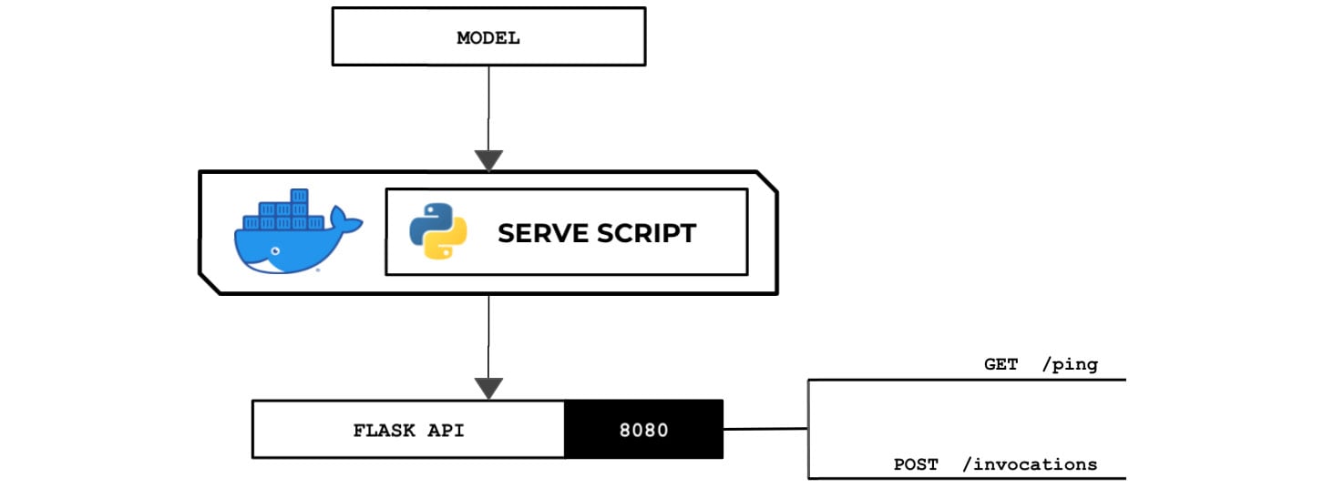
Figure 2.49 – The Python serve script loads and deserializes the model and runs a Flask API server that acts as the inference endpoint

The web server is expected to have the /ping and /invocations endpoints. This standalone Python script will run inside a custom container that allows the Python train and serve scripts to run.

Getting ready

Make sure you have completed the Preparing and testing the train script in Python recipe.

How to do it…

We will start by preparing the serve script:

1. Inside the ml-python directory, double-click the serve file to open it inside the Editor pane:
   

   Figure 2.50 – Locating the empty serve script inside the ml-python directory

   Here, we can see three files under the ml-python directory. Remember that in the Setting up the Python and R experimentation environments recipe, we prepared an empty serve script:

   

   Figure 2.51 – Empty serve file

   In the next couple of steps, we will add the lines of code for the serve script.

2. Add the following code to the serve script to import and initialize the prerequisites:

   #!/usr/bin/env python3
   import numpy as np
   from flask import Flask
   from flask import Response
   from flask import request
       
   from joblib import dump, load

3. Initialize the Flask app. After that, define the get_path() function:

   app = Flask(__name__)
       
       
   PATHS = {
       'hyperparameters': 'input/config/hyperparameters.json',
       'input': 'input/config/inputdataconfig.json',
       'data': 'input/data/',
       'model': 'model/'
   }
       
   def get_path(key):
       return '/opt/ml/' + PATHS[key]

4. Define the load_model() function by adding the following lines of code to the serve script:

   def load_model():
       model = None
       
       filename = get_path('model') + 'model'
       print(filename)
       
       model = load(filename)
       return model

   Note that the filename of the model here is model as we specified this model artifact filename when we saved the model using the dump() function in the Preparing and testing the train script in Python recipe.

   Important note

   Note that it is important to choose the right approach when saving and loading machine learning models. In some cases, machine learning models from untrusted sources may contain malicious instructions that cause security issues such as arbitrary code execution! For more information on this topic, feel free to check out https://joblib.readthedocs.io/en/latest/persistence.html.

5. Define a function that accepts the POST requests for the /invocations route:

   @app.route("/invocations", methods=["POST"])
   def predict():
       model = load_model()
       post_body = request.get_data().decode("utf-8")
       payload_value = float(post_body)
       
       X_test = np.array(
           [payload_value]
       ).reshape(-1, 1)
       y_test = model.predict(X_test)
       
       return Response(
           response=str(y_test[0]), 
           status=200
       )

   This function has five parts: loading the trained model using the load_model() function, reading the POST request data using the request.get_data() function and storing it inside the post_body variable, transforming the prediction payload into the appropriate structure and type using the float(), np.array(), and reshape() functions, making a prediction using the predict() function, and returning the prediction value inside a Response object.

   Important note

   Note that the implementation of the predict() function in the preceding code block can only handle predictions involving single payload values. At the same time, it can't handle different types of input similar to how built-in algorithms handle CSV, JSON, and other types of request formats. If you need to provide support for this, additional lines of code need to be added to the implementation of the predict() function.

6. Prepare the /ping route and handler by adding the following lines of code to the serve script:

   @app.route("/ping")
   def ping():
       return Response(response="OK", status=200)

7. Finally, use the app.run() method and bind the web server to port 8080:

   app.run(host="0.0.0.0", port=8080)

   Tip

   You can access a working copy of the serve script file in this book's GitHub repository: https://github.com/PacktPublishing/Machine-Learning-with-Amazon-SageMaker-Cookbook/blob/master/Chapter02/ml-python/serve.

8. Create a new Terminal in the bottom pane, below the Editor pane:
   

   Figure 2.52 – New Terminal

   Here, we can see a Terminal tab already open. If you need to create a new one, simply click the plus (+) sign and then click New Terminal. We will run the next few commands in this Terminal tab.

9. Install the Flask framework using pip. We will use Flask for our inference API endpoint:

   pip3 install flask

10. Navigate to the ml-python directory:

    cd /home/ubuntu/environment/opt/ml-python

11. Make the serve script executable using chmod:

    chmod +x serve

12. Test the serve script using the following command:

    ./serve

    This should start the Flask app, as shown here:

    

    Figure 2.53 – Running the serve script

    Here, we can see that our serve script has successfully run a flask API web server on port 8080.

    Finally, we will trigger this running web server.

13. Open a new Terminal window:
    

    Figure 2.54 – New Terminal

    As we can see, we are creating a new Terminal tab as the first tab is already running the serve script.

14. In a separate Terminal window, test the ping endpoint URL using the curl command:

    SERVE_IP=localhost
    curl http://$SERVE_IP:8080/ping

    Running the previous line of code should yield an OK message from the /ping endpoint.

15. Test the invocations endpoint URL using the curl command:

    curl -d "1" -X POST http://$SERVE_IP:8080/invocations

    We should get a value similar or close to 881.3428400857507 after invoking the invocations endpoint.

Now, let's see how this works!

How it works…

In this recipe, we prepared the serve script in Python. The serve script makes use of the Flask framework to generate an API that allows GET requests for the /ping route and POST requests for the /invocations route.

The serve script is expected to load the model file(s) from the /opt/ml/model directory and run a backend API server inside the custom container. It should provide a /ping route and an /invocations route. With these in mind, our bare minimum Flask application template may look like this:

from flask import Flask
app = Flask(__name__)
    
@app.route("/ping")
def ping():
    return <RETURN VALUE>
    
@app.route("/invocations", methods=["POST"])
def predict():
    return <RETURN VALUE>

The app.route() decorator maps a specified URL to a function. In this template code, whenever the /ping URL is accessed, the ping() function is executed. Similarly, whenever the /invocations URL is accessed with a POST request, the predict() function is executed.

Note

Take note that we are free to use any other web framework (for example, the Pyramid Web Framework) for this recipe. So long as the custom container image has the required libraries for the script that's been installed, then we can import and use these libraries in our script files.

In this recipe, we will prepare a Dockerfile for the custom Python container image. We will make use of the train and serve scripts that we prepared in the previous recipes. After that, we will run the docker build command to prepare the image before pushing it to an Amazon ECR repository.

Tip

Wait! What's a Dockerfile? It's a text document containing the directives (commands) used to prepare and build a container image. This container image then serves as the blueprint when running containers. Feel free to check out https://docs.docker.com/engine/reference/builder/ for more information on Dockerfiles.

Getting ready

Make sure you have completed the Preparing and testing the serve script in Python recipe.

How to do it…

The initial steps in this recipe focus on preparing a Dockerfile. Let's get started:

1. Double-click the Dockerfile file in the file tree to open it in the Editor pane. Make sure that this is the same Dockerfile that's inside the ml-python directory:
   

   Figure 2.55 – Opening the Dockerfile inside the ml-python directory

   Here, we can see a Dockerfile inside the ml-python directory. Remember that we created an empty Dockerfile in the Setting up the Python and R experimentation environments recipe. Clicking it in the file tree should open an empty file in the Editor pane:

   

   Figure 2.56 – Empty Dockerfile in the Editor pane

   Here, we have an empty Dockerfile. In the next step, we will update this by adding three lines of code.

2. Update Dockerfile with the following block of configuration code:

   FROM arvslat/amazon-sagemaker-cookbook-python-base:1
   COPY train /usr/local/bin/train
   COPY serve /usr/local/bin/serve

   Here, we are planning to build on top of an existing image called amazon-sagemaker-cookbook-python-base. This image already has a few prerequisites installed. These include the Flask, pandas, and Scikit-learn libraries so that you won't have to worry about getting the installation steps working properly in this recipe. For more details on this image, check out https://hub.docker.com/r/arvslat/amazon-sagemaker-cookbook-python-base:

   

   Figure 2.57 – Docker Hub page for the base image

   Here, we can see the Docker Hub page for the amazon-sagemaker-cookbook-python-base image.

   Tip

   You can access a working copy of this Dockerfile in the Machine Learning with Amazon SageMaker Cookbook GitHub repository: https://github.com/PacktPublishing/Machine-Learning-with-Amazon-SageMaker-Cookbook/blob/master/Chapter02/ml-python/serve.

   With the Dockerfile ready, we will proceed with using the Terminal until the end of this recipe:

3. You can use a new Terminal tab or an existing one to run the next set of commands:
   

   Figure 2.58 – New Terminal

   Here, we can see how to create a new Terminal. Note that the Terminal pane is under the Editor pane in the AWS Cloud9 IDE.

4. Navigate to the ml-python directory containing our Dockerfile:

   cd /home/ubuntu/environment/opt/ml-python

5. Specify the image name and the tag number:

   IMAGE_NAME=chap02_python
   TAG=1

6. Build the Docker container using the docker build command:

   docker build --no-cache -t $IMAGE_NAME:$TAG .

   The docker build command makes use of what is written inside our Dockerfile. We start with the image specified in the FROM directive and then we proceed by copying the file into the container image.

7. Use the docker run command to test if the train script works:

   docker run --name pytrain --rm -v /opt/ml:/opt/ml $IMAGE_NAME:$TAG train

   Let's quickly discuss some of the different options that were used in this command. The --rm flag makes Docker clean up the container after the container exits. The -v flag allows us to mount the /opt/ml directory from the host system to the /opt/ml directory of the container:

   

   Figure 2.59 – Result of the docker run command (train)

   Here, we can see the results after running the docker run command. It should show logs similar to what we had in the Preparing and testing the train script in Python recipe.

8. Use the docker run command to test if the serve script works:

   docker run --name pyserve --rm -v /opt/ml:/opt/ml $IMAGE_NAME:$TAG serve

   After running this command, the Flask API server starts successfully. We should see logs similar to what we had in the Preparing and testing the serve script in Python recipe:

   

   Figure 2.60 – Result of the docker run command (serve)

   Here, we can see that the API is running on port 8080. In the base image we used, we added EXPOSE 8080 to allow us to access this port in the running container.

9. Open a new Terminal tab:
   

   Figure 2.61 – New Terminal

   As the API is running already in the first Terminal, we have created a new one.

10. In the new Terminal tab, run the following command to get the IP address of the running Flask app:

    SERVE_IP=$(docker network inspect bridge | jq -r ".[0].Containers[].IPv4Address" | awk -F/ '{print $1}')
    echo $SERVE_IP

    We should get an IP address that's equal or similar to 172.17.0.2. Of course, we may get a different IP address value.

11. Next, test the ping endpoint URL using the curl command:

    curl http://$SERVE_IP:8080/ping

    We should get an OK after running this command.

12. Finally, test the invocations endpoint URL using the curl command:

    curl -d "1" -X POST http://$SERVE_IP:8080/invocations

    We should get a value similar or close to 881.3428400857507 after invoking the invocations endpoint.

At this point, it is safe to say that the custom container image we have prepared in this recipe is ready. Now, let's see how this works!

How it works…

In this recipe, we built a custom container image using the Dockerfile configuration we specified. When you have a Dockerfile, the standard set of steps would be to use the docker build command to build the Docker image, authenticate with ECR to gain the necessary permissions, use the docker tag command to tag the image appropriately, and use the docker push command to push the Docker image to the ECR repository.

Let's discuss what we have inside our Dockerfile. If this is your first time hearing about Dockerfiles, they are simply text files containing commands to build the image. In our Dockerfile, we did the following:

• We used arvslat/amazon-sagemaker-cookbook-python-base as the base image. Check out https://hub.docker.com/repository/docker/arvslat/amazon-sagemaker-cookbook-python-base for more details about this image.
• We copied the train and serve scripts to the /usr/local/bin directory inside the container image. These scripts are executed when we use docker run.

Using the arvslat/amazon-sagemaker-cookbook-python-base image as the base image allowed us to write a shorter Dockerfile that focuses only on copying the train and serve files to the directory inside the container image. Behind the scenes, we have already pre-installed the flask, pandas, scikit-learn, and joblib packages, along with their prerequisites, inside this container image so that we will not run into issues when building the custom container image. Here is a quick look at the Dockerfile file we used as the base image that we are using in this recipe:

FROM ubuntu:18.04
    
RUN apt-get -y update
RUN apt-get install -y python3.6
RUN apt-get install -y --no-install-recommends python3-pip
RUN apt-get install -y python3-setuptools
    
RUN ln -s /usr/bin/python3 /usr/bin/python & \
    ln -s /usr/bin/pip3 /usr/bin/pip
    
RUN pip install flask
RUN pip install pandas
RUN pip install scikit-learn
RUN pip install joblib
    
WORKDIR /usr/local/bin
EXPOSE 8080

In this Dockerfile, we can see that we are using Ubuntu:18.04 as the base image. Note that we can use other base images as well, depending on the libraries and frameworks we want to be installed in the container image.

Once we have the container image built, the next step will be to test if the train and serve scripts will work inside the container once we use docker run. Getting the IP address of the running container may be the trickiest part, as shown in the following block of code:

SERVE_IP=$(docker network inspect bridge | jq -r ".[0].Containers[].IPv4Address" | awk -F/ '{print $1}')

We can divide this into the following parts:

• docker network inspect bridge: This provides detailed information about the bridge network in JSON format. It should return an output with a structure similar to the following JSON value:

  [
      {
          ...
          "Containers": {
              "1b6cf4a4b8fc5ea5...": {
                  "Name": "pyserve",
                  "EndpointID": "ecc78fb63c1ad32f0...",
                  "MacAddress": "02:42:ac:11:00:02",
                  "IPv4Address": "172.17.0.2/16",
                  "IPv6Address": ""
              }
          },
          ...
      }
  ]

• jq -r ".[0].Containers[].IPv4Address": This parses through the JSON response value from docker network inspect bridge. Piping this after the first command would yield an output similar to 172.17.0.2/16.
• awk -F/ '{print $1}': This splits the result from the jq command using the / separator and returns the value before /. After getting the AA.BB.CC.DD/16 value from the previous command, we get AA.BB.CC.DD after using the awk command.

Once we have the IP address of the running container, we can ping the /ping and /invocations endpoints, similar to how we did in the Preparing and testing the serve script in Python recipe.

In the next recipes in this chapter, we will use this custom container image when we do training and deployment with the SageMaker Python SDK.

In the previous recipe, we have prepared and built the custom container image using the docker build command. In this recipe, we will push the custom container image to an Amazon ECR repository. If this is your first time hearing about Amazon ECR, it is simply a fully managed container registry that helps us manage our container images.

After pushing the container image to an Amazon ECR repository, we can use this image for training and deployment in the Using the custom Python algorithm container image for training and inference with Amazon SageMaker Local Mode recipe.

Getting ready

Here are the prerequisites for this recipe:

• This recipe continues from the Building and testing the custom Python algorithm container image recipe.
• You will need the necessary permissions to manage the Amazon ECR resources if you're using an AWS IAM user with a custom URL.

How to do it…

The initial steps in this recipe focus on creating the ECR repository. Let's get started:

1. Use the search bar in the AWS Console to navigate to the Elastic Container Registry console. Click Elastic Container Registry when it appears in the search results:
   

   Figure 2.62 – Navigating to the ECR console

   As you can see, we can use the search bar to quickly navigate to the Elastic Container Registry service. If we type in ecr, the Elastic Container Registry service in the search results may come up in third or fourth place.

2. Click the Create repository button:
   

   Figure 2.63 – Create repository button

   Here, the Create repository button is at the top right of the screen.

3. In the Create repository form, specify a Repository name. Use the value of $IMAGE_NAME from the Building and testing the custom Python algorithm container image recipe. In this case, we will use chap02_python:
   

   Figure 2.64 – Create repository form

   Here, we have the Create repository form. For Visibility settings, we will choose Private and set the Tag immutability configuration to Disabled.

4. Scroll down until you see the Create repository button. Leave the other configuration settings as-is and click Create repository:
   

   Figure 2.65 – Create repository button

   As we can see, the Create repository button is at the bottom of the page.

5. Click chap02_python:
   

   Figure 2.66 – Link to the ECR repository page

   Here, we have a link under the Repository name column. Clicking this link should redirect us to the repository's details page.

6. Click View push commands:
   

   Figure 2.67 – View push commands button (upper right)

   As we can see, the View push commands button is at the top right of the page, beside the Edit button.

7. You may optionally copy the first command, aws ecr get-login-password …, from the dialog box.
   

   Figure 2.68 – Push commands dialog box

   Here, we can see multiple commands that we can use. We will only need the first one (aws ecr get-login-password …). Click the icon with two overlapping boxes on the right-hand side of the code box to copy the entire line to the clipboard.

8. Navigate back to the AWS Cloud9 environment IDE and create a new Terminal. You may also reuse an existing one:
   

   Figure 2.69 – New Terminal

   The preceding screenshot shows us how to create a new Terminal. Click the green plus button and then select New Terminal from the list of options. Note that the green plus button is directly under the Editor pane.

9. Navigate to the ml-python directory:

   cd /home/ubuntu/environment/opt/ml-python

10. Get the account ID using the following commands:

    ACCOUNT_ID=$(aws sts get-caller-identity | jq -r ".Account")
    echo $ACCOUNT_ID

11. Specify the IMAGE_URI value and use the ECR repository name we specified while creating the repository in this recipe. In this case, we will run IMAGE_URI="chap02_python":

    IMAGE_URI="<insert ECR Repository URI>"
    TAG="1"

12. Authenticate with Amazon ECR so that we can push our Docker container image to an Amazon ECR repository in our account later:

    aws ecr get-login-password --region us-east-1 | docker login --username AWS --password-stdin $ACCOUNT_ID.dkr.ecr.us-east-1.amazonaws.com

    Important note

    Note that we have assumed that our repository is in the us-east-1 region. Feel free to modify the region in the command if needed. This applies to all the commands in this chapter.

13. Use the docker tag command:

    docker tag $IMAGE_URI:$TAG $ACCOUNT_ID.dkr.ecr.us-east-1.amazonaws.com/$IMAGE_URI:$TAG

14. Push the image to the Amazon ECR repository using the docker push command:

    docker push $ACCOUNT_ID.dkr.ecr.us-east-1.amazonaws.com/$IMAGE_URI:$TAG

    At this point, our custom container image should now be successfully pushed into the ECR repository.

Now that we have completed this recipe, we can proceed with using this custom container image for training and inference with SageMaker in the next recipe. But before that, let's see how this works!

How it works…

In the previous recipe, we used the docker build command to prepare the custom container image. In this recipe, we created an Amazon ECR repository and pushed our custom container image to the repository. With Amazon ECR, we can store, manage, share, and run custom container images anywhere. This includes using these container images in SageMaker during training and deployment.

When pushing the custom container image to the Amazon ECR repository, we need the account ID, region, repository name, and tag. Once we have these, the docker push command will look something like this:

docker push <ACCOUNT_ID>.dkr.ecr.<REGION>.amazonaws.com/<REPOSITORY NAME>:<TAG>

When working with container image versions, make sure to change the version number every time you modify this Dockerfile and push a new version to the ECR repository. This will be helpful when you need to use a previous version of a container image.

In this recipe, we will perform the training and deployment steps in Amazon Sagemaker using the custom container image we pushed to the ECR repository in the Pushing the custom Python algorithm container image to an Amazon ECR repository recipe. In Chapter 1, Getting Started with Machine Learning Using Amazon SageMaker, we used the image URI of the container image of the built-in Linear Learner. In this chapter, we will use the image URI of the custom container image instead.

The following diagram shows how SageMaker passes data, files, and configuration to and from each custom container when we use the fit() and predict() functions with the SageMaker Python SDK:

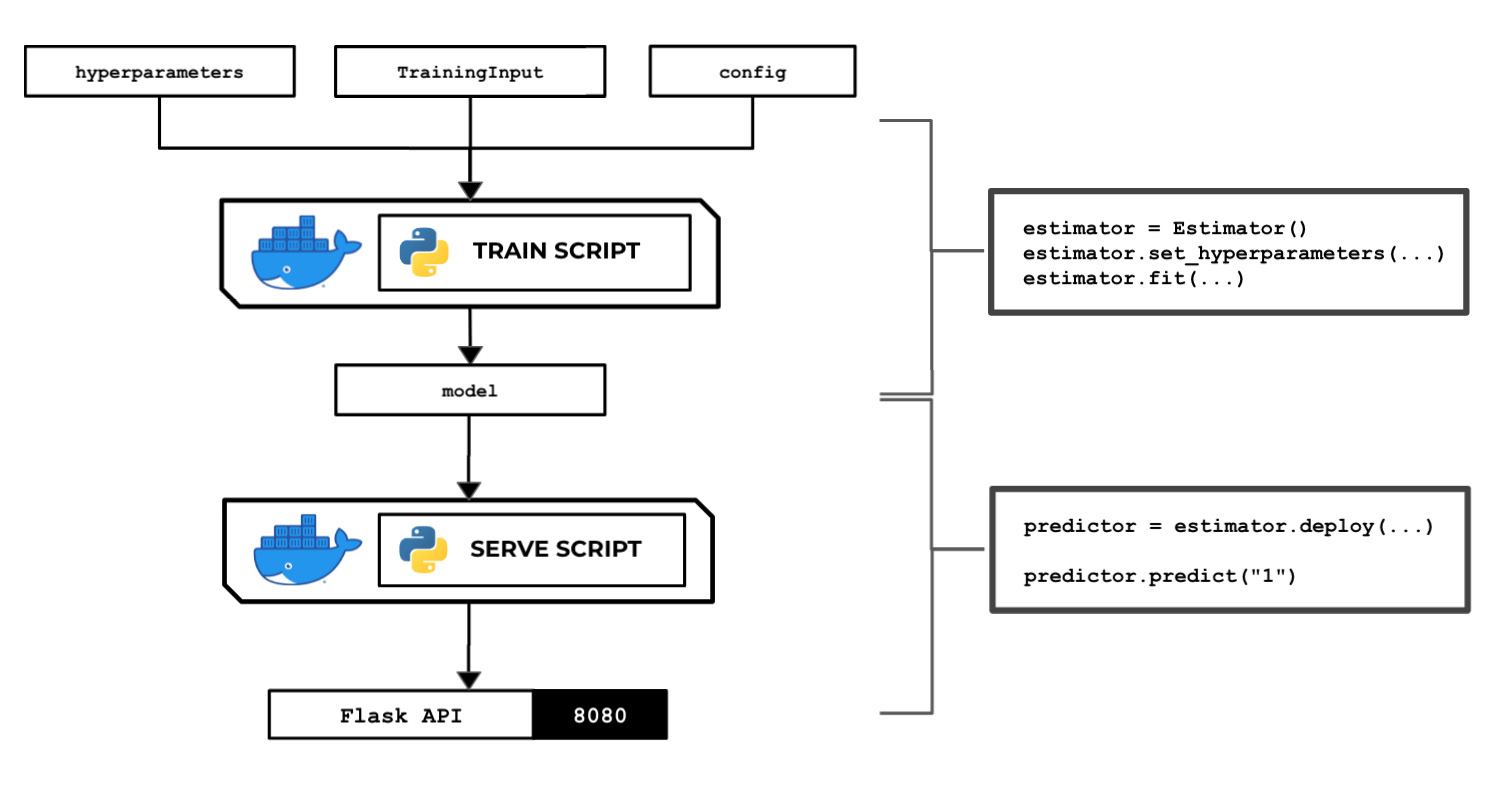
Figure 2.70 – The train and serve scripts inside the custom container make use of the hyperparameters, input data, and config specified using the SageMaker Python SDK

We will also take a look at how to use local mode in this recipe. This capability of SageMaker allows us to test and emulate the CPU and GPU training jobs inside our local environment. Using local mode is useful while we are developing, enhancing, and testing our custom algorithm container images and scripts. We can easily switch to using ML instances that support the training and deployment steps once we are ready to roll out the stable version of our container image.

Once we have completed this recipe, we will be able to run training jobs and deploy inference endpoints using Python with custom train and serve scripts inside custom containers.

Getting ready

Here are the prerequisites for this recipe:

• This recipe continues from the Pushing the custom Python algorithm container image to an Amazon ECR repository recipe.
• We will use the SageMaker Notebook instance from the Launching an Amazon SageMaker Notebook instance and preparing the prerequisites recipe of Chapter 1, Getting Started with Machine Learning Using Amazon SageMaker.

How to do it…

The first couple of steps in this recipe focus on preparing the Jupyter Notebook using the conda_python3 kernel:

1. Inside your SageMaker Notebook instance, create a new directory called chapter02 inside the my-experiments directory. As shown in the following screenshot, we can perform this step by clicking the New button and then choosing Folder (under Other):
   

   Figure 2.71 – New > Folder

   This will create a directory named Untitled Folder.

2. Click the checkbox and then click Rename. Change the name to chapter02:
   

   Figure 2.72 – Renaming "Untitled Folder" to "chapter02"

   After that, we should get the desired directory structure, as shown in the preceding screenshot. Now, let's look at the following directory structure:

   

   Figure 2.73 – Directory structure

   This screenshot shows how we want to organize our files and notebooks. As we go through each chapter, we will add more directories using the same naming convention to keep things organized.

3. Click the chapter02 directory to navigate to /my-experiments/chapter02.
4. Create a new notebook by clicking New and then clicking conda_python3:
   

   Figure 2.74 – Creating a new notebook using the conda_python3 kernel

   Now that we have a fresh Jupyter Notebook using the conda_python3 kernel, we will proceed with preparing the prerequisites for the training and deployment steps.

5. In the first cell of the Jupyter Notebook, use pip install to upgrade sagemaker[local]:

   !pip install 'sagemaker[local]' --upgrade

   This will allow us to use local mode. We can use local mode when working with framework images such as TensorFlow, PyTorch, scikit-learn, and MXNet, and custom images we have built ourselves.

   Important note

   Note that we can NOT use local mode in SageMaker Studio. We also can NOT use local mode with built-in algorithms.

6. Specify the bucket name where the training_data.csv file is stored. Use the bucket name we created in the Preparing the Amazon S3 bucket and the training dataset for the linear regression experiment recipe of Chapter 1, Getting Started with Machine Learning Using Amazon SageMaker:

   s3_bucket = "<insert bucket name here>"
   prefix = "chapter01"

   Note that our training_data.csv file should exist already inside the S3 bucket and should have the following path:

   s3://<S3 BUCKET NAME>/<PREFIX>/input/training_data.csv

7. Set the variable values for training_s3_input_location and training_s3_output_location:

   training_s3_input_location = \ f"s3://{s3_bucket}/{prefix}/input/training_data.csv"
   training_s3_output_location = \ f"s3://{s3_bucket}/{prefix}/output/custom/"

8. Import the SageMaker Python SDK and check its version:

   import sagemaker
   sagemaker.__version__

   We should get a value equal to or near 2.31.0 after running the previous block of code.

9. Set the value of the container image. Use the value from the Pushing the custom Python algorithm container image to an Amazon ECR repository recipe. The container variable should be set to a value similar to <ACCOUNT_ID>.dkr.ecr.us-east-1.amazonaws.com/chap02_python:1. Make sure to replace <ACCOUNT_ID> with your AWS account ID:

   container="<insert image uri and tag here>"

   To get the value of <ACCOUNT_ID>, run ACCOUNT_ID=$(aws sts get-caller-identity | jq -r ".Account") and then echo $ACCOUNT_ID inside a Terminal. Remember that we performed this step in the Pushing the custom Python algorithm container image to an Amazon ECR repository recipe, so you should get the same value for ACCOUNT_ID.

10. Import a few prerequisites such as role and session. You will probably notice one of the major differences between this recipe and the recipes in Chapter 1, Getting Started with Machine Learning Using Amazon SageMaker – the usage of LocalSession. The LocalSession class allows us to use local mode in the training and deployment steps:

    import boto3
    from sagemaker import get_execution_role 
    role = get_execution_role()
    from sagemaker.local import LocalSession
    session = LocalSession()
    session.config = {'local': {'local_code': True}}

11. Initialize the TrainingInput object for the train data channel:

    from sagemaker.inputs import TrainingInput
    train = TrainingInput(training_s3_input_location, content_type="text/csv")

    Now that we have the prerequisites, we will proceed with initializing Estimator and using the fit() and predict() functions.

12. Initialize Estimator and use container, role, session, and training_s3_output_location as the parameter values when initializing the Estimator object:

    estimator = sagemaker.estimator.Estimator(
        container,
        role, 
        instance_count=1, 
        instance_type='local',
        output_path=training_s3_output_location,
        sagemaker_session=session)

    Here, we set the instance_type value to local and the sagemaker_session value to session (which is a LocalSession object). This means that when we run the fit() function later, the training job is performed locally and no ML instances will be provisioned for the training job.

    Important note

    If we want to perform the training job in a dedicated ML instance, simply replace the instance_type value with ml.m5.xlarge (or an alternative ML instance type) and the sagemaker_session value with a Session object. To make sure that we do not encounter training job name validation issues (as we used an underscore in the ECR repository name), specify the base_job_name parameter value with the appropriate value when initializing Estimator.

13. Set a few dummy hyperparameters by using the set_hyperparameters() function. Behind the scenes, these values will passed to the hyperparameters.json file inside the /opt/ml/input/config directory, which will be loaded and used by the train script when we run the fit() function later:

    estimator.set_hyperparameters(a=1, b=2, c=3)

14. Start the training job using fit():

    estimator.fit({'train': train})

    This should generate a set of logs similar to the following:

    

    Figure 2.75 – Using fit() with local mode

    Here, we can see a similar set of logs are generated when we run the train script inside our experimentation environment. As with the Training your first model in Python recipe of Chapter 1, Getting Started with Machine Learning Using Amazon SageMaker, the fit() command will prepare an instance for the duration of the training job to train the model. In this recipe, we are using local mode, so no instances are created.

    Important note

    To compare this to what we did in Chapter 1, Getting Started with Machine Learning Using Amazon SageMaker, we used the fit() function with the Model class from Chapter 1, while we used the fit() function with the Estimator class in this chapter. We can technically use either of these but in this recipe, we went straight ahead and used the fit() function after the Estimator object was initialized, without initializing a separate Model object.

15. Use the deploy() function to deploy the inference endpoint:

    predictor = estimator.deploy(
        initial_instance_count=1, 
        instance_type='local', 
        endpoint_name="custom-local-py-endpoint")

    As we are using local mode, no instances are created and the container is run inside the SageMaker Notebook instance:

    

    Figure 2.76 – Using deploy() with local mode

    As we can see, we are getting log messages in a similar way to how we got them in the Building and testing the custom Python algorithm container image recipe. This means that if we couldn't get the container running in that recipe, then we will not get the container running in this recipe either.

16. Once the endpoint is ready, we can use the predict() function to test if the inference endpoint is working as expected. This will trigger the /invocations endpoint behind the scenes and pass a value of "1" in the POST body:

    predictor.predict("1")

    This should yield a set of logs similar to the following:

    

    Figure 2.77 – Using predict() with local mode

    Here, we can see the logs from the API web server that was launched by the serve script inside the container. We should get a value similar or close to '881.3428400857507'. We will get the return value of the sample invocations endpoint we have coded in a previous recipe:

    @app.route("/invocations", methods=["POST"])
    def predict():
        model = load_model()
        ...
        return Response(..., status=200)

    If we go back and check the Preparing and testing the serve script in Python recipe in this chapter, we will see that we have full control of how the invocations endpoint works by modifying the code inside the predict() function in the serve script. We have copied a certain portion of the function in the preceding code block for your convenience.

17. Use delete_endpoint() to delete the local prediction endpoint:

    predictor.delete_endpoint()

    We should get a message similar to the following:

Figure 2.78 – Using delete_endpoint() with local mode

As we can see, using delete_endpoint() will result in the Gracefully stopping… message. Given that we are using local mode in this recipe, the delete_endpoint() function will stop the running API server in the SageMaker Notebook instance. If local mode is not used, the SageMaker inference endpoint and the ML compute instance(s) that support it will be deleted.

Now, let's check how this works!

How it works…

In this recipe, we used the custom container image we prepared in the previous sections while training and deploying Python, instead of the built-in algorithms of SageMaker. All the steps are similar to the ones we followed for the built-in algorithms; the only changes you will need to take note of are the container image, the input parameters, and the hyperparameters.

Take note that we have full control of the hyperparameters we can specify in Estimator as this depends on the hyperparameters that are expected by our custom script. If you need a more realistic example of these hyperparameters, here are the hyperparameters from Chapter 1, Getting Started with Machine Learning Using Amazon SageMaker:

estimator.set_hyperparameters(
    predictor_type='regressor',
    mini_batch_size=4)

In this example, the hyperparameters.json file, which contains the following content, is created when the fit() function is called:

{"predictor_type": "regressor", "mini_batch_size": 4}

The arguments we can use and configure in this recipe are more or less the same as the ones we used for the built-in algorithms of SageMaker. The only major difference is that we are using the container image URI of our ECR repository instead of the container image URI for the built-in algorithms.

When we're using our custom container images, we have the option to use local mode when performing training and deployment. With local mode, no additional instances outside of the SageMaker Notebook instance are created. This allows us to test if the custom container image is working or not, without having to wait for a couple of minutes compared to using real instances (for example, ml.m5.xlarge). Once things are working as expected using local mode, we can easily switch to using the real instances by replacing session and instance_type in Estimator.

In this recipe, we will write a custom train script in R that allows us to inspect the input and configuration parameters set by Amazon SageMaker during the training process. The following diagram shows the train script inside the custom container, which makes use of the hyperparameters, input data, and configuration specified in the Estimator instance using the SageMaker Python SDK and the reticulate package:

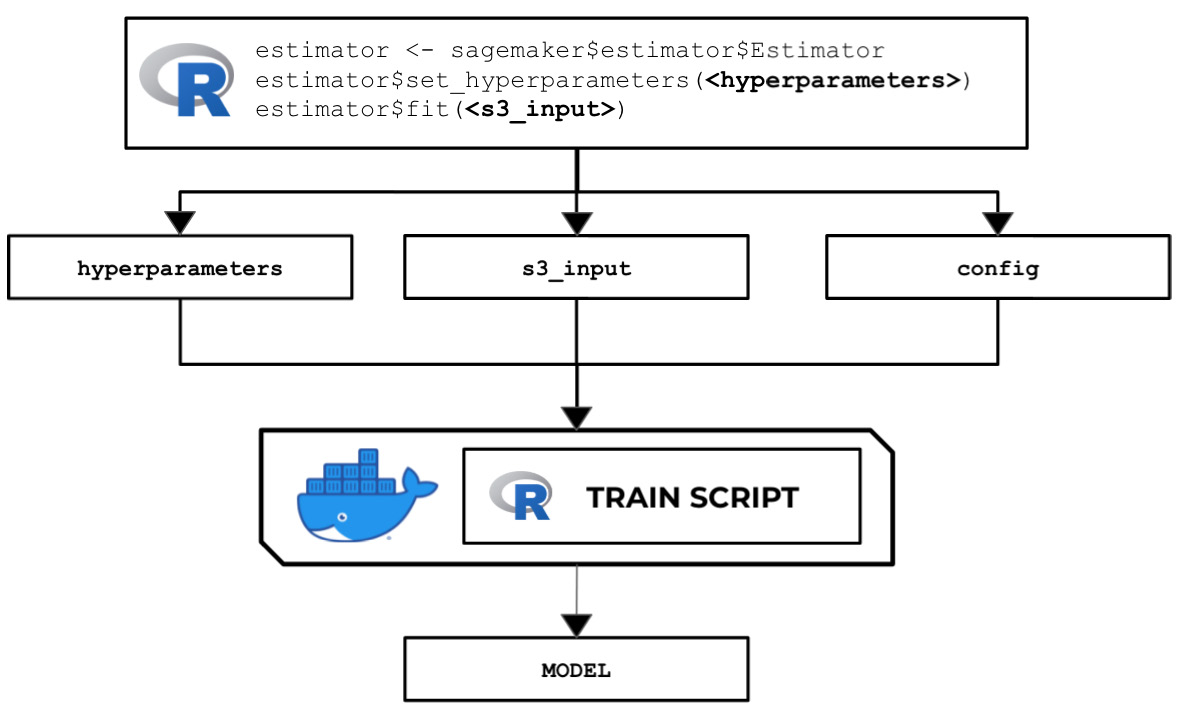
Figure 2.79 – The R train script inside the custom container makes use of the input parameters, configuration, and data to train and output a model

There are several options when running a training job – use a built-in algorithm, use a custom train script and custom Docker images, or use a custom train script and prebuilt Docker images. In this recipe, we will focus on the second option, where we will prepare and test a bare minimum training script in R that builds a linear model for a specific regression problem.

Once we have finished working on this recipe, we will have a better understanding of how SageMaker works behind the scenes. We will see where and how to load and use the configuration and arguments we have specified in the SageMaker Python SDK Estimator instance.

Important note

Later on, you will notice a few similarities between the Python and R recipes in this chapter. What is critical here is noticing and identifying both major and subtle differences in certain parts of the Python and R recipes. For example, when working with the serve script in this chapter, we will be dealing with two files in R (api.r and serve) instead of one in Python (serve). As we will see in the other recipes of this book, working on the R recipes will help us have a better understanding of the internals of SageMaker's capabilities, as there is a big chance that we will have to prepare custom solutions to solve certain requirements. As we get exposed to more machine learning requirements, we will find that there are packages in R for machine learning without direct counterparts in Python. That said, we must be familiar with how to get custom R algorithm code working in SageMaker. Stay tuned for more!

Getting ready

Make sure you have completed the Setting up the Python and R experimentation environments recipe.

How to do it...

The first set of steps in this recipe focus on preparing the train script. Let's get started:

1. Inside the ml-r directory, double-click the train file to open it inside the Editor pane:
   

   Figure 2.80 – Empty ml-r/train file

   Here, we have an empty train file. In the lower-right-hand corner of the Editor pane, you can change the syntax highlight settings to R.

2. Add the following lines of code to start the train script in order to import the required packages and libraries:

   #!/usr/bin/Rscript
   library("rjson")

3. Define the prepare_paths() function, which we will use to initialize the PATHS variable. This will help us manage the paths of the primary files and directories used in the script:

   prepare_paths <- function() {
       keys <- c('hyperparameters', 
                 'input', 
                 'data',
                 'model')
       
       values <- c('input/config/hyperparameters.json', 
                   'input/config/inputdataconfig.json', 
                   'input/data/',
                   'model/')
       
       paths <- as.list(values)
       names(paths) <- keys
       
       return(paths);
   } 
       
   PATHS <- prepare_paths()

   This function allows us to initialize the PATHS variable with a dictionary-like data structure where we can get the absolute paths of the required file.

4. Next, define the get_path() function, which makes use of the PATHS variable from the previous step:

   get_path <- function(key) {
       output <- paste('/opt/ml/', PATHS[[key]],
                       sep="")
       
       return(output);
   }

   When referring to the location of a specific file, such as hyperparameters.json, we will use get_path('hyperparameters') instead of the absolute path.

5. Next, add the following lines of code just after the get_path() function definition from the previous step. These functions will be used to load and print the contents of the JSON files we will work with later:

   load_json <- function(target_file) {
       result <- fromJSON(file = target_file)
   }
   print_json <- function(target_json) {
       print(target_json)
   }

6. After that, define the inspect_hyperparameters() and list_dir_contents() functions after the print_json() function definition:

   inspect_hyperparameters <- function() {
       hyperparameters_json_path <- get_path(
           'hyperparameters'
       )
       print(hyperparameters_json_path)
       hyperparameters <- load_json(
           hyperparameters_json_path
       )
       print(hyperparameters)
   }
   list_dir_contents <- function(target_path) {
       print(list.files(target_path))
   }

   The inspect_hyperparameters() function inspects the contents of the hyperparameters.json file inside the /opt/ml/input/config directory. The list_dir_contents() function, on the other hand, displays the contents of a target directory.

7. Define the inspect_input() function. It will help us inspect the contents of inputdataconfig.json inside the /opt/ml/input/config directory:

   inspect_input <- function() {
       input_config_json_path <- get_path('input')
       print(input_config_json_path)
       input_config <- load_json(
           input_config_json_path
       )
       print_json(input_config)
       
       for (key in names(input_config)) {
           print(key)
           
           input_data_dir <- paste(get_path('data'), 
                                   key, '/', sep="")
           print(input_data_dir)
           list_dir_contents(input_data_dir)
       }
   }

   This will be used to list the contents of the training input directory inside the main() function later.

8. Define the load_training_data() function:

   load_training_data <- function(input_data_dir) {
       print('[load_training_data]')
       files <- list_dir_contents(input_data_dir)
       training_data_path <- paste0(
           input_data_dir, files[[1]])
       print(training_data_path)
       
       df <- read.csv(training_data_path, header=FALSE)
       colnames(df) <- c("y","X")
       print(df)
       return(df)
   }

   This function can be divided into two parts – preparing the specific path pointing to the CSV file containing the training data and reading the contents of the CSV file using the read.csv() function. The return value of this function is an R DataFrame (a two-dimensional table-like structure).

9. Next, define the get_input_data_dir() function:

   get_input_data_dir <- function() {
       print('[get_input_data_dir]')
       key <- 'train'
       input_data_dir <- paste0(
           get_path('data'), key, '/')
       
       return(input_data_dir)
   }

10. After that, define the train_model() function:

    train_model <- function(data) {
        model <- lm(y ~ X, data=data)    
        print(summary(model))
        return(model)
    }

    This function makes use of the lm() function to fit and prepare linear models, which can then be used for regression tasks. It accepts a formula such as y ~ X as the first parameter value and the training dataset as the second parameter value.

    Note

    Formulas in R involve a tilde symbol (~) and one or more independent variables at the right of the tilde (~), such as X1 + X2 + X3. In the example in this recipe, we only have one variable on the right-hand side of the tilde (~), meaning that we will only have a single predictor variable for this model. On the left-hand side of the tilde (~) is the dependent variable that we are trying to predict using the predictor variable(s). That said, the y ~ X formula simply expresses a relationship between the predictor variable, X, and the y variable we are trying to predict. Since we are dealing with the same dataset as we did for the recipes in Chapter 1, Getting Started with Machine Learning Using Amazon SageMaker, the y variable here maps to monthly_salary, while X maps to management_experience_months.

11. Define the save_model() function:

    save_model <- function(model) {
        print('[save_model]')
        filename <- paste0(get_path('model'), 'model')
        print(filename)
        saveRDS(model, file=filename)
        print('Model Saved!')
    }

    Here, we make use of the saveRDS() function, which accepts an R object and writes it to a file. In this case, we will accept a trained model object and save it inside the /opt/ml/model directory.

12. Define the main() function, as shown here. This function triggers the functions defined in the previous steps:

    main <- function() {
        inspect_hyperparameters()
        inspect_input()
        input_data_dir = get_input_data_dir()
        print(input_data_dir)
        data <- load_training_data(input_data_dir)
        model <- train_model(data)
        save_model(model)
    }

    This main() function can be divided into four parts – inspecting the hyperparameters and the input, loading the training data, training the model using the train_model() function, and saving the model using the save_model() function.

13. Finally, call the main() function at the end of the script:

    main()

    Tip

    You can access a working copy of the train file in the Machine Learning with Amazon SageMaker Cookbook GitHub repository: https://github.com/PacktPublishing/Machine-Learning-with-Amazon-SageMaker-Cookbook/blob/master/Chapter02/ml-r/train.

    Now that we are done with the train script, we will use the Terminal to perform the last set of steps in this recipe. The last set of steps focus on installing a few script prerequisites.

14. Open a new Terminal:
    

    Figure 2.81 – New Terminal

    Here, we can see how to create a new Terminal tab. We simply click the plus (+) button and then choose New Terminal.

15. Check the version of R in the Terminal:

    R --version

    Running this line of code should return a similar set of results to what is shown here:

    

    Figure 2.82 – Result of the R --version command in the Terminal

    Here, we can see that our environment is using R version 3.4.4.

16. Install the rjson package:

    sudo R -e "install.packages('rjson',repos='https://cloud.r-project.org')"

    The rjson package provides the utilities for handling JSON data in R.

17. Use the following commands to make the train script executable and then run the train script:

    cd /home/ubuntu/environment/opt/ml-r
    chmod +x train
    ./train

    Running the previous lines of code will yield results similar to what is shown here:

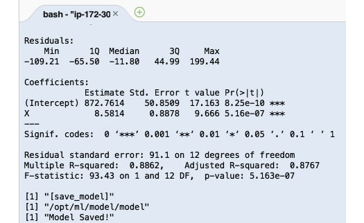
Figure 2.83 – R train script output

Here, we can see the logs that were produced by the train script. Once the train script has been successfully executed, we expect the model files to be stored inside the /opt/ml/model directory.

At this point, we have finished preparing and testing the train script. Now, let's see how this works!

How it works…

The train script in this recipe demonstrates how the input and output values are passed around between the SageMaker API and the custom container. It also performs a fairly straightforward set of steps to train a linear model using the training data provided.

When you are required to work on a more realistic example, the train script will do the following:

• Load and use a few environment variables using the Sys.getenv() function in R. We can load environment variables set by SageMaker automatically, such as TRAINING_JOB_NAME and TRAINING_JOB_ARN.
• Load the contents of the hyperparameters.json file using the fromJSON() function.
• Load the contents of the inputdataconfig.json file using the fromJSON() function. This file contains the properties of each of the input data channels, such as the file type and usage of the file or pipe mode.
• Load the data file(s) inside the /opt/ml/input/data directory. Take note that there's a parent directory named after the input data channel in the path before the actual files themselves. An example of this would be /opt/ml/input/data/<channel name>/<filename>.
• Perform model training using the hyperparameters and training data that was loaded in the previous steps.
• Save the model inside the /opt/ml/model directory:

  saveRDS(model, file="/opt/ml/model/model.RDS")

• We can optionally evaluate the model using the validation data and log the results.

Now that have finished preparing the train script in R, let's quickly discuss some possible solutions we can prepare using what we learned in this recipe.

There's more…

It is important to note that we are free to use any algorithm in the train script to train our model. This level of flexibility gives us an edge once we need to work on more complex examples. Here is a quick example of what the train function may look like if the neuralnet R package is used in the train script:

train <- function(df.training_data, hidden_layers=4) {
    model <- neuralnet(
        label ~ ., 
        df.training_data, 
        hidden=c(hidden_layers,1),
        linear.output = FALSE, 
        threshold=0.02,
        stepmax=1000000,
        act.fct = "logistic")
    return(model)
}

In this example, we allow the number of hidden layers to be set while we are configuring the Estimator object using the set_hyperparameters() function. The following example shows how to implement a train function to prepare a time series forecasting model in R:

train <- function(data) {
    model <- snaive(data) 
    print(summary(model))
    return(model)
}

Here, we simply used the snaive() function from the forecast package to prepare the model. Of course, we are free to use other functions as well, such as ets() and auto.arima() from the forecast package.

In this recipe, we will create a serve script using R that runs an inference API using the plumber package. This API loads the model during initialization and uses the model to perform predictions during endpoint invocation.

The following diagram shows the expected behavior of the R serve script that we will prepare in this recipe. The R serve script loads the model file from the /opt/ml/model directory and runs a plumber web server on port 8080:

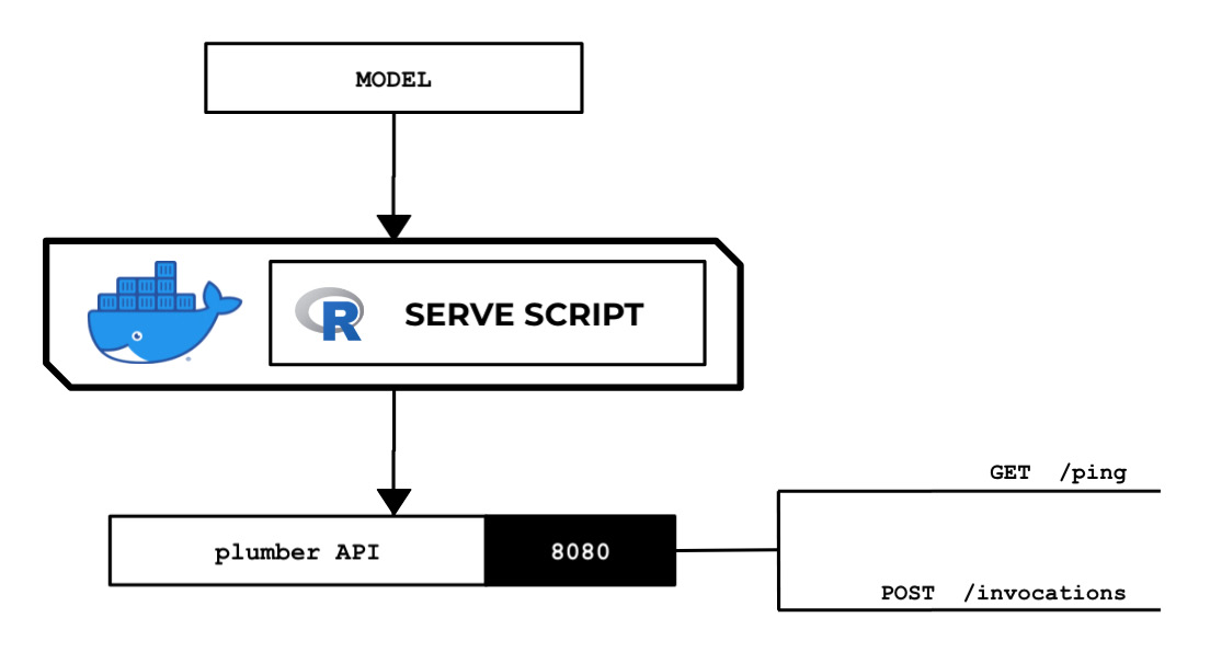
Figure 2.84 – The R serve script loads and deserializes the model and runs a plumber API server that acts as the inference endpoint

The web server is expected to have the /ping and /invocations endpoints. This standalone R backend API server will run inside a custom container later.

Getting ready

Make sure you have completed the Preparing and testing the train script in R recipe.

How to do it...

We will start by preparing the api.r file:

1. Double-click the api.r file inside the ml-r directory in the file tree:
   

   Figure 2.85 – An empty api.r file inside the ml-r directory

   Here, we can see four files under the ml-r directory. Remember that we created an empty api.r file in the Setting up the Python and R experimentation environments recipe:

   

   Figure 2.86 – Empty api.r file

   In the next couple of steps, we will add a few lines of code inside this api.r file. Later, we will learn how to use the plumber package to generate an API from this api.r file.

2. Define the prepare_paths() function, which we will use to initialize the PATHS variable. This will help us manage the paths of the primary files and directories used in the script. This function allows us to initialize the PATHS variable with a dictionary-like data structure, which we can use to get the absolute paths of the required files:

   prepare_paths <- function() {
       keys <- c('hyperparameters', 
                 'input', 
                 'data',
                 'model')
       values <- c('input/config/hyperparameters.json', 
                   'input/config/inputdataconfig.json', 
                   'input/data/',
                   'model/')
       paths <- as.list(values)
       names(paths) <- keys
       return(paths);
   }
       
   PATHS <- prepare_paths()

3. Next, define the get_path() function, which makes use of the PATHS variable from the previous step:

   get_path <- function(key) {
       output <- paste(
           '/opt/ml/', PATHS[[key]], sep="")
       return(output);
   }

4. Create the following function (including the comments), which responds with "OK" when triggered from the /ping endpoint:

   #* @get /ping
   function(res) {
     res$body <- "OK"
     return(res)
   }

   The line containing #* @get /ping tells plumber that we will use this function to handle the GET requests with the /ping route.

5. Define the load_model() function:

   load_model <- function() {
     model <- NULL
     filename <- paste0(get_path('model'), 'model')
     print(filename)
     model <- readRDS(filename)
     return(model)
   }

6. Define the following /invocations function, which loads the model and uses it to perform a prediction on the input value from the request body:

   #* @post /invocations
   function(req, res) {
     print(req$postBody)
     model <- load_model()
     payload_value <- as.double(req$postBody)
     X_test <- data.frame(payload_value)
     colnames(X_test) <- "X"
     
     print(summary(model))
     y_test <- predict(model, X_test)
     output <- y_test[[1]]
     print(output)
     
     res$body <- toString(output)
     return(res)
   }

   Here, we loaded the model using the load_model() function, transformed and prepared the input payload before passing it to the predict() function, used the predict() function to perform the actual prediction when given an X input value, and returned the predicted value in the request body.

   Tip

   You can access a working copy of the api.r file in the Machine Learning with Amazon SageMaker Cookbook GitHub repository: https://github.com/PacktPublishing/Machine-Learning-with-Amazon-SageMaker-Cookbook/blob/master/Chapter02/ml-r/api.r.

   Now that the api.r file is ready, let's prepare the serve script:

7. Double-click the serve file inside the ml-r directory in the file tree:
   

   Figure 2.87 – The serve file inside the ml-r directory

   It should open an empty serve file, similar to what is shown in the following screenshot:

   

   Figure 2.88 – The serve file inside the ml-r directory

   We will add the necessary code to this empty serve file in the next set of steps.

8. Start the serve script with the following lines of code. Here, we are loading the plumber and here packages:

   #!/usr/bin/Rscript
   suppressWarnings(library(plumber))
   library('here')

   The here package provides utility functions to help us easily build paths to files (for example, api.r).

9. Add the following lines of code to start the plumber API server:

   path <- paste0(here(), "/api.r")
   pr <- plumb(path)
   pr$run(host="0.0.0.0", port=8080)

   Here, we used the plumb() and run() functions to launch the web server. It is important to note that the web server endpoint needs to run on port 8080 for this to work correctly.

   Tip

   You can access a working copy of the serve script in the Machine Learning with Amazon SageMaker Cookbook GitHub repository: https://github.com/PacktPublishing/Machine-Learning-with-Amazon-SageMaker-Cookbook/blob/master/Chapter02/ml-r/serve.

10. Open a new Terminal tab:
    

    Figure 2.89 – Locating the Terminal

    Here, we see that a Terminal tab is already open. If you need to create a new one, simply click the plus (+) sign and then click New Terminal.

11. Install libcurl4-openssl-dev and libsodium-dev using apt-get install. These are some of the prerequisites for installing the plumber package:

    sudo apt-get install -y --no-install-recommends libcurl4-openssl-dev
    sudo apt-get install -y --no-install-recommends libsodium-dev

12. Install the here package:

    sudo R -e "install.packages('here',repos='https://cloud.r-project.org')"

    The here package helps us get the string path values we need to locate specific files (for example, api.r). Feel free to check out https://cran.r-project.org/web/packages/here/index.html for more information.

13. Install the plumber package:

    sudo R -e "install.packages('plumber',repos='https://cloud.r-project.org')"

    The plumber package allows us to generate an HTTP API in R. For more information, feel free to check out https://cran.r-project.org/web/packages/plumber/index.html.

14. Navigate to the ml-r directory:

    cd /home/ubuntu/environment/opt/ml-r

15. Make the serve script executable using chmod:

    chmod +x serve

16. Run the serve script:

    ./serve

    This should yield log messages similar to the following ones:

    

    Figure 2.90 – The serve script running

    Here, we can see that our serve script has successfully run a plumber API web server on port 8080.

    Finally, we must trigger this running web server.

17. Open a new Terminal tab:
    

    Figure 2.91 – New Terminal

    Here, we are creating a new Terminal tab as the first tab is already running the serve script.

18. Set the value of the SERVE_IP variable to localhost:

    SERVE_IP=localhost

19. Check if the ping endpoint is available with curl:

    curl http://$SERVE_IP:8080/ping

    Running the previous line of code should yield an OK from the /ping endpoint.

20. Test the invocations endpoint with curl:

    curl -d "1" -X POST http://$SERVE_IP:8080/invocations

    We should get a value close to 881.342840085751.

Now, let's see how this works!

How it works…

In this recipe, we prepared the serve script in R. The serve script makes use of the plumber package to serve an API that allows GET requests for the /ping route and POST requests for the /invocations route. The serve script is expected to load the model file(s) from the specified model directory and run a backend API server inside the custom container. This should provide a /ping route and an /invocations route.

Compared to its Python recipe counterpart, we are dealing with two files instead of one as that's how we used plumber in this recipe:

• The api.r file defines what the API looks like and how it behaves.
• The serve script uses the api.r file to initialize and launch a web server using the plumb() function from the plumber package. Note that with Flask, there is no need to create a separate file to define the API routes.

When working with the plumber package, we start with an R file describing how the API will behave (for example, api.r). This R file follows the following format:

#* @get /ping
function(res) {
  res$body <- "OK"
  return(<RETURN VALUE>)
}
     
#* @post /invocations
function(req, res) {
  return(<RETURN VALUE>)
}

Once this R file is ready, we simply create an R script that makes use of the plumb() function from the plumber package. This will launch a web server using the configuration and behavior coded in the api.r file:

pr <- plumb(<PATH TO API.R>)
pr$run(host="0.0.0.0", port=8080)

With this, whenever the /ping URL is accessed, the mapped function defined in the api.r file is executed. Similarly, whenever the /invocations URL is accessed with a POST request, the corresponding mapped function is executed. For more information on the plumber package, feel free to check out https://www.rplumber.io/.

In the previous two recipes, we prepared and tested the train, serve, and api.r files. With these ready, we can now proceed with crafting the Dockerfile and building the custom algorithm container image.

Tip

Wait! What's a Dockerfile? It is a text document containing the directives (commands) used to prepare and build a container image. This container image then serves as the blueprint when running containers. Feel free to check out https://docs.docker.com/engine/reference/builder/ for more information.

In this recipe, we will prepare a Dockerfile for the custom R container image. We will make use of the api.r file, as well as the train and serve scripts we prepared in the Preparing and testing the train script in R and Preparing and testing the serve script in R recipes. After that, we will use the docker build command to prepare the image before pushing it to an Amazon ECR repository.

Getting ready

Make sure you have completed the Preparing and testing the serve script in R recipe.

How to do it...

The initial steps in this recipe focus on preparing the Dockerfile. Let's get started:

1. Double-click the Dockerfile file in the file tree to open it in the Editor pane. Make sure that this is the same Dockerfile that's inside the ml-r directory:
   

   Figure 2.92 – Opening the Dockerfile inside the ml-r directory

   Here, we can see that there's a Dockerfile inside the ml-r directory. Remember that we created an empty Dockerfile in the Setting up the Python and R experimentation environments recipe. Clicking on it in the file tree should open an empty file in the Editor pane:

   

   Figure 2.93 – Empty Dockerfile

   Here, we have an empty Dockerfile. In the next step, we will update this by adding four lines of code.

2. Update the Dockerfile with the following block of configuration code:

   FROM arvslat/amazon-sagemaker-cookbook-r-base:1
   COPY train /usr/local/bin/train
   COPY serve /usr/local/bin/serve
   COPY api.r /usr/local/bin/api.r

   Here, we are planning to build on top of an existing image called amazon-sagemaker-cookbook-r-base. This image already has a few prerequisites installed. These include the rjson, here, and plumber packages so that you don't have to worry about getting the installation steps working properly in this recipe. For more details on this image, check out https://hub.docker.com/r/arvslat/amazon-sagemaker-cookbook-r-base:

   

   Figure 2.94 – Docker Hub page for the amazon-sagemaker-cookbook-r-base image

   Here, we can see the Docker Hub page for the amazon-sagemaker-cookbook-r-base image.

   Tip

   You can access a working copy of this Dockerfile in the Amazon SageMaker Cookbook GitHub repository: https://github.com/PacktPublishing/Machine-Learining-with-Amazon-SageMaker-Cookbook/blob/master/Chapter02/ml-r/Dockerfile.

   With our Dockerfile ready, we will proceed by using the Terminal until the end of this recipe.

3. You may use a new Terminal tab or an existing one to run the next set of commands:
   

   Figure 2.95 – New Terminal

   The preceding screenshot shows how to create a new Terminal. Note that the Terminal pane is right under the Editor pane in the AWS Cloud9 IDE.

4. Navigate to the ml-python directory containing our Dockerfile:

   cd /home/ubuntu/environment/opt/ml-r

5. Specify the image name and the tag number:

   IMAGE_NAME=chap02_r
   TAG=1

6. Build the Docker container using the docker build command:

   docker build --no-cache -t $IMAGE_NAME:$TAG .

   The docker build command makes use of what is written inside our Dockerfile. We start with the image specified in the FROM directive and then proceed by copying the file files into the container image.

7. Use the docker run command to test if the train script works:

   docker run --name rtrain --rm -v /opt/ml:/opt/ml $IMAGE_NAME:$TAG train

   Let's quickly discuss some of the different options that are used in this command. The --rm flag makes Docker clean up the container after the container exits, while the -v flag allows us to mount the /opt/ml directory from the host system to the /opt/ml directory of the container:

   

   Figure 2.96 – Result of the docker run command (train)

   Here, we can see the logs and results after running the docker run command.

8. Use the docker run command to test if the serve script works:

   docker run --name rserve --rm -v /opt/ml:/opt/ml $IMAGE_NAME:$TAG serve

   After running this command, the plumber API server will start successfully, as shown in the following screenshot:

   

   Figure 2.97 – Result of the docker run command (serve)

   Here, we can see that the API is running on port 8080. In the base image we used, we added EXPOSE 8080 to allow us to access this port in the running container.

9. Open a new Terminal tab:
   

   Figure 2.98 – New Terminal

   As the API is running already in the first Terminal, we have created a new Terminal here.

10. In the new Terminal tab, run the following command to get the IP address of the running Plumber API:

    SERVE_IP=$(docker network inspect bridge | jq -r ".[0].Containers[].IPv4Address" | awk -F/ '{print $1}')
    echo $SERVE_IP

    What happened here? Check out the How it works… section of this recipe for a detailed explanation of what happened in the previous block of code! In the meantime, let's think of this line as using multiple commands to get the IP address of the running API server. We should get an IP address equal or similar to 172.17.0.2. Of course, we may get a different IP address value altogether.

11. Next, test the ping endpoint URL using the curl command:

    curl http://$SERVE_IP:8080/ping

    We should get an OK after running this command.

12. Finally, test the invocations endpoint URL using the curl command:

    curl -d "1" -X POST http://$SERVE_IP:8080/invocations

    We should get a value similar or close to 881.342840085751 after invoking the invocations endpoint.

Now, let's see how this works!

How it works…

In this recipe, we built a custom container image with our Dockerfile. In our Dockerfile, we did the following:

• We used the arvslat/amazon-sagemaker-cookbook-r-base image as the base image. Check out https://hub.docker.com/repository/docker/arvslat/amazon-sagemaker-cookbook-r-base for more details on this image.
• We copied the train, serve, and api.r files to the /usr/local/bin directory inside the container image. These scripts are executed when we use docker run.

Using the arvslat/amazon-sagemaker-cookbook-r-base image as the base image allowed us to write a shorter Dockerfile that focuses only on copying the train, serve, and api.r files to the directory inside the container image. Behind the scenes, we have already pre-installed the rjson, plumber, and here packages, along with their prerequisites, inside this container image so that we will not run into issues when building the custom container image. Here is a quick look at the Dockerfile file that was used for the base image that we are using in this recipe:

FROM r-base:4.0.2
RUN apt-get -y update 
RUN apt-get install -y --no-install-recommends wget
RUN apt-get install -y --no-install-recommends libcurl4-openssl-dev
RUN apt-get install -y --no-install-recommends libsodium-dev
    
RUN R -e "install.packages('rjson',repos='https://cloud.r-project.org')"
RUN R -e "install.packages('plumber',repos='https://cloud.r-project.org')"
RUN R -e "install.packages('here',repos='https://cloud.r-project.org')"
    
ENV PATH "/opt/ml:$PATH"
WORKDIR /usr/local/bin
EXPOSE 8080

In this Dockerfile, we can see that we are using r-base:4.0.2 as the base image. If we were to use a higher version, there's a chance that the plumber package will not install properly, which is why we had to stick with a lower version of this base image.

With these potential blockers out of the way, we were able to build a custom container image in a short amount of time. In the Using the custom R algorithm container image for training and inference with Amazon SageMaker Local Mode recipe of this chapter, we will use this custom container image when we do training and deployment with reticulate so that we can use the SageMaker Python SDK with our R code.

In the previous recipe, we prepared and built the custom container image using the docker build command. In this recipe, we will push the custom container image to an Amazon ECR repository. If this is your first time hearing about Amazon ECR, it is simply a fully managed container registry that helps us manage our container images. After pushing the container image to an Amazon ECR repository, we will use this image for training and deployment in the Using the custom R algorithm container image for training and inference with Amazon SageMaker Local Mode recipe.

Getting ready

Here are the prerequisites for this recipe:

• This recipe continues from the Building and testing the custom R algorithm container image recipe.
• Permission to manage the Amazon ECR resources if you're using an AWS IAM user with a custom URL.

How to do it...

The initial steps in this recipe focus on creating the ECR repository. Let's get started:

1. Use the search bar in the AWS Console to navigate to the Elastic Container Registry console. Click Elastic Container Registry when you see it in the search results:
   

   Figure 2.99 – Navigating to the ECR console

   As we can see, we can use the search bar to quickly navigate to the Elastic Container Registry service.

2. Click the Create repository button:
   

   Figure 2.100 – Create repository button

   Here, the Create repository button is at the top right of the screen.

3. In the Create repository form, specify a Repository name. Use the value of $IMAGE_NAME from the Building and testing the custom R algorithm container image recipe. In this case, we will use chap02_r:
   

   Figure 2.101 – Create repository form

   Here, we have the Create repository form. For Visibility settings, we chose Private and we set the Tag immutability configuration to Disabled.

4. Scroll down until you see the Create repository button. Leave the other configuration settings as-is and click Create repository:
   

   Figure 2.102 – Create repository button

   Finally, to complete the repository creation process, click the Create repository button at the bottom of the page.

5. Click chap02_r:
   

   Figure 2.103 – Link to the ECR repository page

   Here, we have a link under the Repository name column. Clicking this link should redirect us to a page containing details about the repository.

6. Click View push commands:
   

   Figure 2.104 – View push commands button (upper right)

   The View push commands button can be found at the top right of the page.

7. You can optionally copy the first command, aws ecr get-login-password …, from the dialog box:
   

   Figure 2.105 – Push commands dialog box

   Here, we can see multiple commands that we can use. We will only need the first one (aws ecr get-login-password …). Click the icon with two overlapping boxes at the right-hand side of the code box to copy the entire line to the clipboard.

8. Navigate back to the AWS Cloud9 environment IDE and create a new Terminal. You can also reuse an existing one:
   

   Figure 2.106 – New Terminal

   The preceding screenshot shows us how to create a new Terminal. We click the green plus button and then select New Terminal from the list of options. Note that the green plus button is right under the Editor pane.

9. Navigate to the ml-r directory:

   cd /home/ubuntu/environment/opt/ml-r

10. Get the account ID using the following commands:

    ACCOUNT_ID=$(aws sts get-caller-identity | jq -r ".Account")
    echo $ACCOUNT_ID

11. Specify the IMAGE_URI value and use the ECR repository name we specified while creating the repository in this recipe. In this case, we will run IMAGE_URI="chap02_r":

    IMAGE_URI="<insert ECR Repository URI>"
    TAG="1"

12. Authenticate with Amazon ECR so that we can push our Docker container image to an Amazon ECR repository in our account later:

    aws ecr get-login-password --region us-east-1 | docker login --username AWS --password-stdin $ACCOUNT_ID.dkr.ecr.us-east-1.amazonaws.com

    Important note

    Note that we have assumed that our repository is in the us-east-1 region. Feel free to modify this region in the command if needed. This applies to all the commands in this chapter.

13. Use the docker tag command:

    docker tag $IMAGE_URI:$TAG $ACCOUNT_ID.dkr.ecr.us-east-1.amazonaws.com/$IMAGE_URI:$TAG

14. Push the image to the Amazon ECR repository using the docker push command:

    docker push $ACCOUNT_ID.dkr.ecr.us-east-1.amazonaws.com/$IMAGE_URI:$TAG

Now that we have completed this recipe, we can proceed with using this custom algorithm container image with SageMaker in the next recipe. But before that, let's see how this works!

How it works…

In the Building and testing the custom R algorithm container image recipe, we used docker build to prepare the custom container image. In this recipe, we created an Amazon ECR repository and pushed our custom container image to it. We also used the docker push command to push the custom container image we built to the ECR repository.

Important note

Don't forget to include the api.r file inside the container when writing this Dockerfile and running the build step. The Python counterpart recipe copies the train and serve scripts to the /opt/ml directory inside the container, while the R recipe copies the train, serve, and api.r files to the /opt/ml directory. If the api.r file is not included, the following line in the serve script file will trigger an error and cause the script to fail: pr <- plumb("/opt/ml/api.r").

In the previous recipe, we pushed the custom R container image to an Amazon ECR repository. In this recipe, we will perform the training and deployment steps in Amazon SageMaker using this custom container image. In the first chapter, we used the image URI of the container image of the built-in Linear Learner algorithm. In this chapter, we will use the image URI of the custom container image instead:

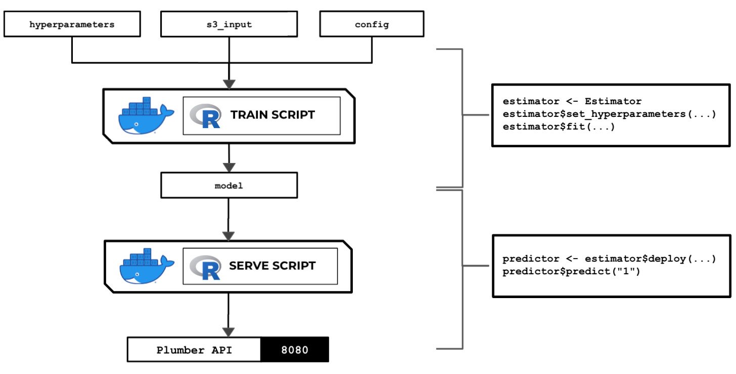
Figure 2.107 – The train and serve scripts inside the custom container make use of the hyperparameters, input data, and config specified using the SageMaker Python SDK

The preceding diagram shows how SageMaker passes data, files, and configuration to and from each custom container when we use the fit() and predict() functions in our R code, which we do with the reticulate package and the SageMaker Python SDK.

We will also look at how to use local mode in this recipe. This capability of SageMaker allows us to test and emulate the CPU and GPU training jobs inside our local environment. Using local mode is useful while we are developing, enhancing, and testing our custom algorithm container images and scripts. We can easily switch to using ML instances that support the training and deployment steps once we are ready to roll out the stable version of our container image.

Once we have completed this recipe, we will be able to run training jobs and deploy inference endpoints using R with custom train and serve scripts inside custom containers.

Getting ready

Here are the prerequisites for this recipe:

• This recipe continues from the Pushing the custom R algorithm container image to an Amazon ECR repository recipe.
• We will use the SageMaker Notebook instance from the Launching an Amazon SageMaker Notebook instance and preparing the prerequisites recipe of Chapter 1, Getting Started with Machine Learning Using Amazon SageMaker.

How to do it...

The first couple of steps in this recipe focus on preparing the Jupyter Notebook using the R kernel. Let's get started:

1. Inside your SageMaker Notebook instance, create a new directory called chapter02 inside the my-experiments directory if it does not exist yet:
   

   Figure 2.108 – Preferred directory structure

   The preceding screenshot shows how we want to organize our files and notebooks. As we go through each chapter, we will add more directories using the same naming convention to keep things organized.

2. Click the chapter02 directory to navigate to /my-experiments/chapter02.
3. Create a new notebook by clicking New and then clicking R:
   

   Figure 2.109 – Creating a new notebook using the R kernel

   The preceding screenshot shows how to create a new Jupyter Notebook using the R kernel.

   Now that we have a fresh Jupyter Notebook using the R kernel, we will proceed with preparing the prerequisites for the training and deployment steps.

4. Prepare the cmd function, which will help us run the Bash commands in the subsequent steps:

   cmd <- function(bash_command) {
       output <- system(bash_command, intern=TRUE)
       last_line = ""
       for (line in output) { 
           cat(line)
           cat("\n")
           last_line = line 
       }
       return(last_line) 
   }

   Given that we are using the R kernel, we will not be able to use the ! prefix to run Bash commands. Instead, we have created a cmd() function that helps us perform a similar operation. This cmd() function makes use of the system() function to invoke system commands.

5. Next, let's use the cmd function to run the pip install command to install and upgrade sagemaker[local]:

   cmd("pip install 'sagemaker[local]' --upgrade")

   This will allow us to use local mode. We can use local mode when working with framework images such as TensorFlow, PyTorch, and MXNet and custom container images we build ourselves.

   Important note

   At the time of writing, we can't use local mode in SageMaker Studio. We also can't use local mode with built-in algorithms.

6. Specify the values for s3.bucket and s3.prefix. Make sure that you set the s3.bucket value to the name of the S3 bucket we created in the Preparing the Amazon S3 bucket and the training dataset for the linear regression experiment recipe of Chapter 1, Getting Started with Machine Learning Using Amazon SageMaker:

   s3.bucket <- "<insert S3 bucket name here>"
   s3.prefix <- "chapter01"

   Remember that our training_data.csv file should already exist inside the S3 bucket and that it should have the following path:

   s3://<S3 BUCKET NAME>/<PREFIX>/input/training_data.csv

7. Now, let's specify the input and output locations in training.s3_input_location and training.s3_output_location, respectively:

   training.s3_input_location <- paste0('s3://', s3.bucket, '/', s3.prefix, '/input/training_data.csv')
   training.s3_output_location <- paste0('s3://', s3.bucket, '/', s3.prefix, '/output/custom/')

8. Load the reticulate package using the library() function. The reticulate package allows us to use the SageMaker Python SDK and other libraries in Python inside R. This gives us a more powerful arsenal of libraries in R. We can use these with other R packages such as ggplot2, dplyr, and caret:

   library('reticulate')
   sagemaker <- import('sagemaker')

   Tip

   For more information on the reticulate package, feel free to check out the How it works… section at the end of this recipe.

9. Check the SageMaker Python SDK version:

   sagemaker[['__version__']]

   We should get a value equal to or greater than 2.31.0.

10. Set the value of the container image. Use the value from the Pushing the custom R algorithm container image to an Amazon ECR repository recipe. The container variable should be set to a value similar to <ACCOUNT_ID>.dkr.ecr.us-east-1.amazonaws.com/chap02_r:1. Make sure that you replace <ACCOUNT_ID> with your AWS account ID:

    container <- "<insert container image URI here>"

    Tip

    To get the value of <ACCOUNT_ID>, run ACCOUNT_ID=$(aws sts get-caller-identity | jq -r ".Account") and then echo $ACCOUNT_ID inside a Terminal. Remember that we performed this step in the Pushing the custom R algorithm container image to an Amazon ECR repository recipe, so you should get the same value for ACCOUNT_ID.

11. Import a few prerequisites, such as the role and the session. For session, we will use the LocalSession class, which will allow us to use local mode in the training and deployment steps:

    role <- sagemaker$get_execution_role()
    LocalSession <- sagemaker$local$LocalSession
    session <- LocalSession()
    session$config <- list(local=list(local_code=TRUE))

12. Prepare the train input so that it points to the Amazon S3 path with content_type="text/csv":

    TrainingInput <- sagemaker$inputs$TrainingInput
    sagemaker.train_input <- TrainingInput(training.s3_input_location, content_type="text/csv")

    Now that we have the prerequisites ready, we will proceed with initializing Estimator and using the fit() and predict() functions.

13. Initialize Estimator with the relevant arguments, as shown in the following code block. Take note that the container variable contains the Amazon ECR image URI of the custom R container image:

    Estimator <- sagemaker$estimator$Estimator
    estimator <- Estimator(
        container,
        role, 
        instance_count=1L, 
        instance_type="local",
        output_path=training.s3_output_location,
        sagemaker_session=session)

14. Set a few dummy hyperparameters using the set_hyperparameters() function:

    estimator$set_hyperparameters(a=1L, b=2L, c=3L)

    Behind the scenes, these values will be passed to the hyperparameters.json file inside the /opt/ml/input/config directory, which will be loaded and used by the train script when we run the fit() function later.

15. Perform the training step by calling the fit() function with the train argument set to the sagemaker.train_input variable value from the previous step:

    estimator$fit(list(train = sagemaker.train_input))

    Compared to our experiment in Chapter 1, Getting Started with Machine Learning Using Amazon SageMaker, the fit() function in this recipe will run the training job inside the SageMaker Notebook instance because of local mode. Given that we are not using local mode, we are launching ML instances that support the training jobs. As we discussed in Chapter 1, these ML instances are normally deleted automatically after the training jobs have been completed.

    Important note

    Even if we are using local mode, the model files generated by the train script are NOT stored inside the SageMaker notebook instance. The model.tar.gz file that contains the model files is still uploaded to the specified output_path in Amazon S3. You can check the value of estimator$model_data to verify this!

16. Deploy the model using the deploy() function. We set instance_type to 'local' and initial_instance_count to 1L. Note that the L makes the number an explicit integer:

    predictor <- estimator$deploy(
        initial_instance_count=1L,
        instance_type="local",
        endpoint_name="custom-local-r-endpoint"
    )

    Given that we are using local mode, the deploy() function will run the container and the serve script inside the SageMaker Notebook instance.

    Important note

    Note that if we change instance_type to a value such as "ml.m5.xlarge" (in addition to not using the LocalSession object), we will be launching a dedicated ML instance outside the SageMaker Notebook instance for the inference endpoint. Of course, the best practice would be to get things working first using local mode. Once we have ironed out the details and fixed the bugs, we can deploy the model to an inference endpoint supported by a dedicated ML instance.

17. Finally, test the predict() function. This triggers the invocations API endpoint you prepared in the previous step and passes "1" as the parameter value:

    predictor$predict("1")

    We should get a value similar or close to 881.342840085751 after invoking the invocations endpoint using the predict() function. Expect the predicted value here to be similar to what we have in the Building and testing the custom R algorithm container image recipe.

    Now that we have a model and an inference endpoint, we can perform some post-processing, visualization, and evaluation steps using R and packages such as ggplot2, dplyr, and Metrics.

18. Delete the endpoint:

    predictor$delete_endpoint()

    Given that we are using local mode in this recipe, the delete_endpoint() function will stop the running API server in the SageMaker Notebook instance. If local mode is not being used, the SageMaker inference endpoint and the ML compute instance(s) that support it will be deleted.

Now, let's check out how this works!

How it works…

In this recipe, we used the reticulate R package to use the SageMaker Python SDK inside our R code. This will help us train and deploy our machine learning model. Instead of using the built-in algorithms of Amazon SageMaker, we used the custom container image we prepared in the previous recipes.

Note

Feel free to check out the How it works… section of the Using the custom Python algorithm container image for training and inference with Amazon SageMaker Local Mode recipe if you need a quick explanation on how training jobs using custom container images work.

To help us understand this recipe better, here are a few common conversions from Python to R you need to be familiar with when using reticulate:

• Dot (.) to dollar sign ($): estimator.fit() to estimator$fit()
• Python dictionary to R lists: {'train': train} to list(train=train)
• Integer values: 1 to 1L
• Built-in constants: None to NULL, True to TRUE, and False to FALSE

Why spend the effort trying to perform machine learning experiments in R when you can use Python instead? There are a couple of possible reasons for this:

• Research papers and examples written by data scientists using R may use certain packages that do not have proper counterpart libraries in Python.
• Professionals and teams already familiar with the R language and using it for years should be able to get an entire ML experiment to work from end to end, without having to learn another language, especially when under time constraints. This happens a lot in real life, where teams are not easily able to shift from using one language to another due to time constraints and language familiarity.
• Migrating existing code from R to Python may not be practical or possible due to time constraints, as well as differences in the implementation of existing libraries in R and Python.

Other data scientists and ML engineers simply prefer to use R over Python. That said, it is important to be ready with solutions that allow us to use R when performing end-to-end machine learning and machine learning engineering tasks. Refer to the following diagram for a quick comparison of the tools and libraries that are used when performing end-to-end experiments in Python and R:

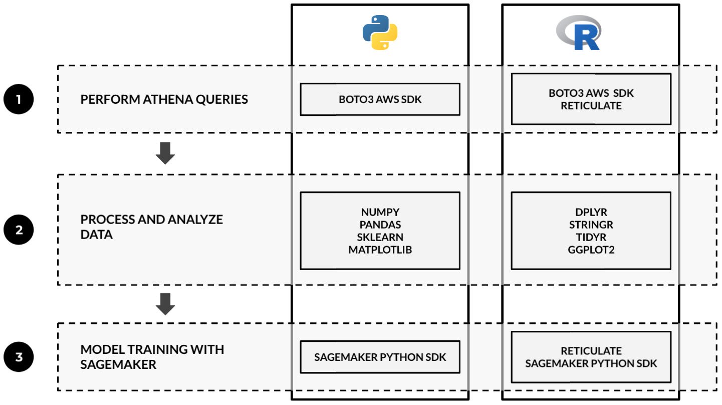
Figure 2.110 – Sample guide for tech stack selection when using Python and R in machine learning experiments

As we can see, we can use the reticulate package to use the Boto3 AWS SDK and the SageMaker Python SDK inside our R code. "Note that the diagram does NOT imply a one-to-one mapping of the presented sample libraries and packages in Python and R." between "As we can see, we can use the reticulate package to use the Boto3 AWS SDK and the SageMaker Python SDK inside our R code." We used Amazon Athena in this example as it is one of the services we can use to help us prepare and query our data before the training phase. With the reticulate package, we can seamlessly use boto3 to execute Athena queries in our R code.

Note

We will take a look at how we can use Amazon Athena with deployed models for data preparation and processing in the Invoking machine learning models with Amazon Athena using SQL queries recipe of Chapter 4, Preparing, Processing, and Analyzing the Data.

When using R, packages such as dplyr, tidyr, and ggplot2 can easily be used with reticulate and the AWS SDKs to solve machine learning requirements from start to finish. That said, machine learning practitioners and teams already using R in their workplace may no longer need to learn another language (for example, Python) and migrate existing code from R to Python.