Regression versus correlation
At the beginning of the chapter, we said that regression analysis is a statistical process for studying the relationship between variables. When considering two or more variables, one can examine the type and intensity of the relationships that exist between them. In the case where two quantitative variables are simultaneously detected for each individual, it is possible to check whether they vary simultaneously and what mathematical relationship exists between them.
The study of such relationships can be conducted through two types of analysis: regression analysis and correlation analysis. Let's understand the differences between these two types of analysis.
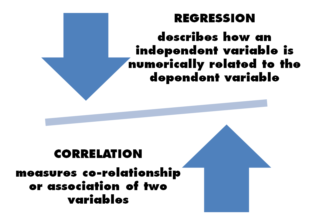
Regression analysis develops a statistical model that can be used to predict the values of a variable, called dependent, or more rarely predict and identify the effect based on the values of the other variable, called independent or explanatory, identified as the cause.
With correlation analysis, we can measure the intensity of the association between two quantitative variables that are usually not directly linked to the cause-effect and easily mediated by at least one third variable, but that vary jointly. In the following figure, the meanings of two analyses are shown:
In many cases, there are variables that tend to covariate, but what more can be said about this? If there is a direct dependency relation between two variables—such as whether a variable (dependent) can be determined as a function of a second variable (independent)—then a regression analysis can be used to understand the degree of the relation. For example, blood pressure depends on the subject's age. The existing data used in regression and mathematical equations is defined. Using these equations, the value of one variable can be predicted for the value of one or more variables. This equation can therefore also be used to extract knowledge from the existing data and to predict the outcomes of observations that have not been seen or tested before.
Conversely, if there is no direct dependency relation between variables—such as none of the two variables causing direct variations in the other—the covariate tendency is measured in correlation. For example, there is no direct relationship between the length and weight of an organism, in the sense that the weight of an organism can increase independently of its length. Correlation measures the association between two variables and it quantifies the strength of the relationship. To do this, it evaluates only the existing data.
To better understand the differences, we will analyze in detail the two examples just suggested. For the first example, we list the blood pressure of subjects of different ages, as shown in the following table:
Age | Blood pressure |
|
|
|
|
|
|
|
|
|
|
|
|
|
|
|
|
|
|
|
|
|
|
A suitable graphical representation called a scatter plot can be used to depict the relationships between quantitative variables detected on the same units. In the following chapters, we will see in practice how to plot a scatter plot, so let's just make sense of the meaning.
We display this data on a scatter plot, as shown in the following figure:
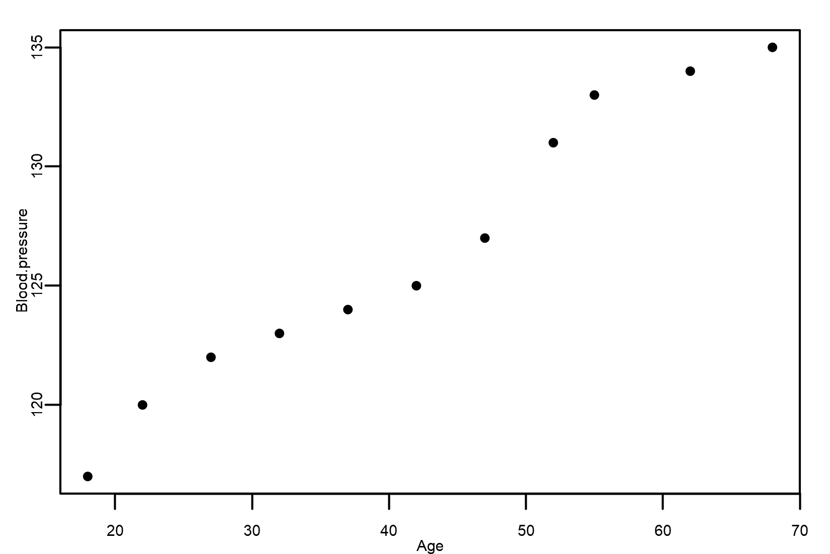
By analyzing the scatter plot, we can answer the following:
- Is there a relationship that can be described by a straight line?
- Is there a relationship that is not linear?
- If the scatter plot of the variables looks similar to a cloud, it indicates that no relationship exists between both variables and one would stop at this point
The scatter plot shows a strong, positive, and linear association between Age and Blood pressure. In fact, as age increases, blood pressure increases.
Let's now look at what happens in the other example. As we have anticipated, there is no direct relationship between the length and weight of an organism, in the sense that the weight of an organism can increase independently of its length.
We can see an example of an organism's population here:
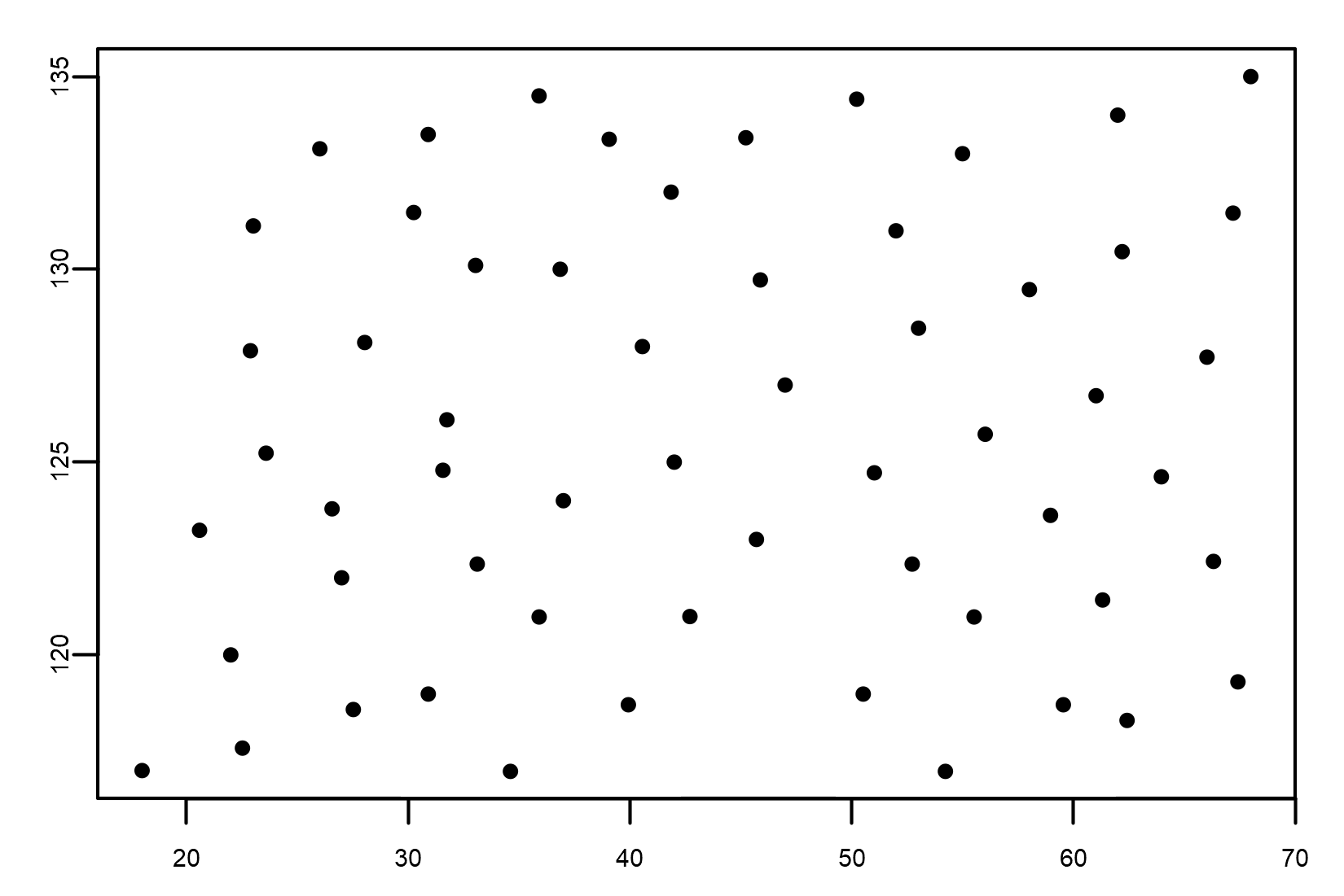
Weight is not related to length; this means that there is no correlation between the two variables, and we conclude that length is responsible for none of the changes in weight.
Correlation provides a numerical measure of the relationship between two continuous variables. The resulting correlation coefficient does not depend on the units of the variables and can therefore be used to compare any two variables regardless of their units.