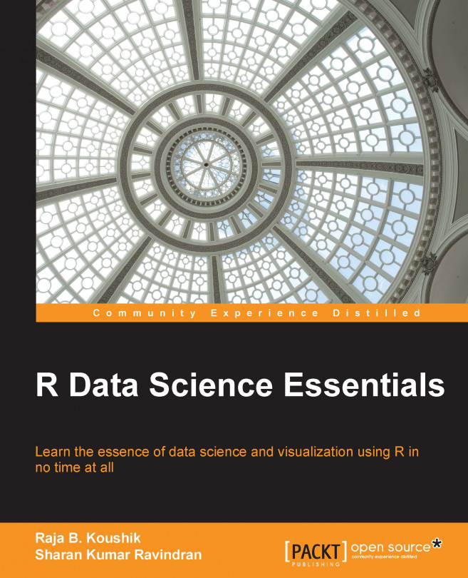
R Data Science Essentials

Chapter 1. Getting Started with R

R is one of the most popular programming languages used in computation statistics, data visualization, and data science. With the increasing number of companies becoming data-driven, the user base of R is also increasing fast. R is supported by over two million users worldwide.

In this book, you will learn how to use R to load data from different sources, carry out fundamental data manipulation techniques, extract the hidden patterns in data through exploratory data analysis, and build complex predictive as well as forecasting models. Finally, you will learn to visualize and communicate the data analysis to the audience. This book is aimed at beginners and intermediate users of R, taking them through the most important techniques in data science that will help them start their data scientist journey.

In this chapter, we will be covering the basic concepts of R such as reading data from different sources, understanding the data format, learning about the preprocessing techniques, and performing basic arithmetic and string operations.

The objective of this chapter is to first help the reader get a hold on to programming in R and know about the basic operations that will be useful for any analysis. In this chapter, we will essentially be exploring the standard techniques that will be used to convert the raw data into a usable format.

The following topics will be covered in this chapter:

Reading data from different sources
Discussing data types in R
Discussing data preprocessing techniques
Performing arithmetic operations on the data
Performing string operations on the data
Discussing control structures in R
Bringing the data into a usable format

Reading data from different sources

Importing data to R is quite simple and can be done from multiple sources. The most common method of importing data to R is through the comma-separated values (CSV) format. The CSV data can be accessed through the read.csv function. This is the simplest way to read the data as it requires just a single line command and the data is ready. Depending on the quality of the data, it may or may not require processing.

data <- read.csv("c:/local-data.csv")

The other function similar to read.csv is read.csv2. This function is also used to read the CSV files but the difference is that read.csv2 is mostly used in the European countries, where comma is used as decimal point and semicolon is used as a separator. Also, the data can be read from R using a few more parameters, such as read.table and read.delim. By default, read.delim is used to read tab-delimited files, and the read.table function can be used to read any file by supplying suitable parameters as the input:

data  <- read.delim("local-data.txt", header=TRUE, sep="\t")
data  <- read.table("local-data.txt", header=TRUE, sep="\t")

Tip

Downloading the example code

You can download the example code files for all Packt books you have purchased from your account at http://www.packtpub.com. If you purchased this book elsewhere, you can visit http://www.packtpub.com/support and register to have the files e-mailed directly to you.

All the preceding functions can take multiple parameters that would explain the data source's format at best. Some of these parameters are as follows:

header: This is a logical value indicating the presence of column names in the file. When it is set to TRUE, it indicates that the column names are present. By default, the value is considered as TRUE.
sep: This defines the separator in the file. By default, the separator is comma for read.csv, tab for read.delim, and white space for the read.table function.
nrows: This specifies the maximum number of rows to read from the file. By default, the entire file will be read.
row.names: This will specify which column should be considered as a row name. When it is set as NULL, the row names will be forced as numbers. This parameter will take the column's position (one represents the first column) as input.
fill: This parameter when set as TRUE can read the data with unequal row lengths and blank fields are implicitly added.

These are some of the common parameters used along with the functions to read the data from a file.

We have so far explored reading data from a delimited file. In addition to this, we can read data in Excel formats as well. This can be achieved using the xlsx or XLConnect packages. We will see how to use one of these packages in order to read a worksheet from a workbook:

install.packages("xlsx")
library(xlsx)
mydata <- read.xlsx("DTH AnalysisV1.xlsx", 1)
head(mydata)

In the preceding code, we first installed the xlsx package that is required to read the Excel files. We loaded the package using the library function, then used the read.xlsx function to read the excel file, and passed an additional parameter, 1, that specifies which sheet to read from the excel file.

Reading data from a database

Apart from reading the data from a local file, R allows us to read the data from different sources and different formats. If we consider any enterprise setup, the data would mostly be present in a database. It will be complicated if we import the data from the database to a local file and then perform the analysis; we should be able to access the data directly from the source. This can be achieved using R.

First, let's see how to access data from a database. In order to read data from a database, we need to establish a connection with the database, which could reside in the local system or a remote server. We can establish the connection to the database using either ODBC or JDBC, which are R packages.

We will have a detailed look at accessing the data from the database using the JDBC method. In order to perform this operation, we need to install the RJDBC and sqldf packages. The RJDBC package is used to establish a connection with the database and the sqldf package is used to write the SQL queries:

install.packages("RJDBC")
library(RJDBC)
install.packages("sqldf")
library(sqldf)

We will now learn to establish a connection with the DB. We need to set up a few things in order to connect with the DB. To use the JDBC connection, we need to download the driver. The downloaded file will depend on the database to which we are going to connect, such as SQL Server, Oracle, or PostgreSQL.

In the following case, we will connect to a SQL server database. The JDBC driver can be downloaded from http://www.microsoft.com/en-in/download/details.aspx?id=11774 in order to provide connectivity. In the following code, we will pass the driver name as well as the location of the JAR file that comes with the download to the JDBC function. The JDBC function creates a new DBI driver that can be used to start the JDBC connection.

drv <- JDBC("com.microsoft.sqlserver.jdbc.SQLServerDriver", "C:/Users/Downloads/Microsoft SQL Server JDBC Driver 3.0/sqljdbc_3.0/enu/sqljdbc4.jar")

By using the dbConnect function, we establish the actual connection with the database. We need to pass the location of the database, username, and password to this function. On the successful execution of the following code, the connection will be established and we can check the connectivity using the dbGetQuery function:

conn <- dbConnect(drv, "jdbc:sqlserver://localhost;database=SAMPLE_DB", "admin", "test")
bin <- dbGetQuery(conn, "select count(*) from  sampletable")

In addition to the relational databases, we can also connect and access the non-relational databases, such as Cassandra, Hadoop, MongoDB, and so on. We will now see how to access data from a Cassandra database. In order to access the data from a Cassandra database, we need to install the RCassandra package. The connection to the database can be made using the RC.connect function. We need to pass the host IP as well as the port number to establish the connection. Then finally, we need to specify the username and password as follows to establish the connection successfully:

library(RCassandra)
conn <- RC.connect(host = "localhost", port = 9160)
RC.login(conn, username = "user", password = "password123")

In Cassandra, the container for the application data is keyspace, which is similar to schema in the relational database. We can use the RC.describe.keyspaces function to get an understanding about the data, and then using the RC.use function, we select keyspace to be used for all the subsequent operations:

RC.describe.keyspaces(conn)
RC.use(conn, keyspace = "sampleDB", cache.def = TRUE)

We can read the data using the following code and once all the readings are done, we can close the connection using RC.close:

a<-RC.read.table(conn, c.family = "Users", convert = TRUE, na.strings = "NA",
              as.is = FALSE, dec = ".")
RC.close(conn)

We can discuss the RMongo package as well as it is quite popular.

Similarly, R has the ability to read data from a table in a website using the XML package. We can also read the data of SAS, SPSS, Stata, and Systat using the Hmisc package for SPSS and SAS and foreign for Stata and Systat.

For more details about the methodology of extracting the data from these sources, find the reference at the following URLs:

While establishing connectivity with a remote system, you could face a few issues related to security and others specific to the R version and package version. Most likely, the common issues would have been discussed in the forum, stackoverflow.

Data types in R

We explored the various ways that we can read the data from R in the previous session. Let's have a look at the various data types that are supported by R. Before going into the details of the data type, we will first explore the variable data types in R.

Variable data types

The common variable data types in R are numerical, integer, character, and logical. We will explore each one of them using R.

Numeric is the default variable type for all the variables holding numerical values in R:

a <- 10
class(a)
[1] "numeric"

In the preceding code, we actually passed an integer to the a variable but it is still being saved in a numeric format.

We can now convert this variable defined as a numeric in R into an integer using the as.integer function:

a <- as.integer(a)
class(a)
[1] "integer"

Similarly, here is a variable of the character and logical types:

name <- "Sharan"
class(name)
[1] "character"

# Logical Type
flag <- TRUE
class(flag)
[1] "logical"

Having explored the variable data types, now we will move up the hierarchy and explore these data types: vector, matrix, list, and dataframe.

A vector is a sequence of elements of a basic data type. It could be a sequence of numeric or logical characters. A vector can't have a sequence of elements with different data types. The following are the examples for the numeric, character, and logical vectors:

v1 <- c(12, 34, -21, 34.5, 100) # numeric vector
class(v1)
 [1] "numeric"
v2 <- c("sam", "paul", "steve",  "mark") # character vector
class(v2)
[1] "character"
v3 <- c(TRUE, FALSE, TRUE, FALSE, TRUE, FALSE) #logical vector
class(v3)
[1] "logical"

Now, let's consider the v1 numeric vector and the v2 character vector, combine these two, and see the resulting vector:

newV <- c(v1,v2)
class(newV)
[1] "character"

We can see that the resultant vector is a character vector; we will see what happened to the numeric elements of the first vector. From the following output, we can see that the numeric elements are now converted into character vectors represented in double quotes, whereas the numeric vector will be represented without any quotes:

newV
 [1] "12"    "34"    "-21"   "34.5"  "100"   "sam"   "paul"  "steve" "mark"

A matrix is a collection of elements that has a two-dimensional representation, that is, columns and rows. A matrix can contain elements of the same data type only. We can create a matrix using the following code. First, we pass the intended row names and column names to the rnames and cnames variables, then using the matrix function, we will create the matrix. We specify the row names and column names using the dimnames parameter:

rnames <- c("R1", "R2", "R3", "R4", "R5")
cnames <- c("C1", "C2", "C3", "C4", "C5")
matdata <-matrix(1:25, nrow=5,ncol=5, dimnames=list(rnames, cnames))
class(matdata)
[1] "matrix"
typeof(matdata)
[1] "integer"
Matdata
C1 C2 C3 C4 C5
R1  1  6 11 16 21
R2  2  7 12 17 22
R3  3  8 13 18 23
R4  4  9 14 19 24
R5  5 10 15 20 25

A list is a sequence of data elements similar to a vector but can hold elements of different datatypes. We will combine the variables that we created in the vector section. As in the following code, these variables hold numeric, character, and logical vectors. Using the list function, we combine them, but their individual data type still holds:

l1 <- list(v1, v2, v3)

typeof(l1)
> l1
[[1]]
[1]  12.0  34.0 -21.0  34.5 100.0

[[2]]
[1] "sam"   "paul"  "steve" "mark" 

[[3]]
[1]  TRUE FALSE  TRUE FALSE  TRUE FALSE

Factors are categorical variables in R, which means that they take values from a limited known set. In case of factor variables, R internally stores an equivalent integer value and maps it to the character string.

A dataframe is similar to the matrix, but in a data frame, the columns can hold data elements of different types. The data frame will be the most commonly used data type for most of the analysis. As any dataset would have multiple data points, each could be of a different type. R comes with a good number of built-in datasets such as mtcars. When we use sample datasets to cover the various examples in the coming chapters, you will get a better understanding about the data types discussed so far.

Data preprocessing techniques

The first step after loading the data to R would be to check for possible issues such as missing data, outliers, and so on, and, depending on the analysis, the preprocessing operation will be decided. Usually, in any dataset, the missing values have to be dealt with either by not considering them for the analysis or replacing them with a suitable value.

To make this clearer, let's use a sample dataset to perform the various operations. We will use a dataset about India named IndiaData. You can find the dataset at https://github.com/rsharankumar/R_Data_Science_Essentials. We will perform preprocessing on the dataset:

data <- read.csv("IndiaData.csv", header = TRUE)
#1. To check the number of Null
sum(is.na(data))
[1] 6831

After reading the dataset, we use the is.na function to identify the presence of NA in the dataset, and then using sum, we get the total number of NAs present in the dataset. In our case, we can see that a large number of rows has NA in it. We can replace the NA with the mean value or we can remove these NA rows.

The following function can be used to replace the NA with the column mean for all the numeric columns. The numeric columns are identified by the sapply(data, is.numeric) function. We will check for the cells that have the NA value, then we identify the mean of these columns using the mean function with the na.rm=TRUE parameter, where the NA values are excluded while computing the mean function:

for (i in which(sapply(data, is.numeric))) {
  data[is.na(data[, i]), i] <- mean(data[, i],  na.rm = TRUE)
}

Alternatively, we can also remove all the NA rows from the dataset using the following code:

newdata <- na.omit(data)

The next major preprocessing activity is to identify the outliers package and deal with it. We can identify the presence of outliers in R by making use of the outliers function. We can use the function outliers only on the numeric columns, hence let's consider the preceding dataset, where the NAs were replaced by the mean values, and we will identify the presence of an outlier using the outliers function. Then, we get the location of all the outliers using the which function and finally, we remove the rows that had outlier values:

install.packages("outliers")
library(outliers)

We identify the outliers in the X2012 column, which can be subsetted using the data$X2012 command:

outlier_tf = outlier(data$X2012,logical=TRUE)
sum(outlier_tf)
[1] 1

#What were the outliers
find_outlier = which(outlier_tf==TRUE,arr.ind=TRUE)
#Removing the outliers
newdata = data[-find_outlier,]
nrow(newdata)

The column from the preceding dataset that was considered in the outlier example had only one outlier and hence we can remove this row from the dataset.

Performing data operations

The following are the different data operations available in R:

Arithmetic operations
String operations
Aggregation operations

Arithmetic operations on the data

In this dataset, we will see the arithmetic operations performed on the data. We can perform various operations such as addition, subtraction, multiplication, division, exponentiation, and modulus. Let's see how these operations are performed in R. Let's first declare two numeric vectors:

a1 <- c(1,2,3,4,5)
b1 <- c(6,7,8,9,10)
c1 <- a1+b1
[1]  7  9 11 13 15
c1 <- b1-a1
 [1] 5 5 5 5 5
c1 <- b1*a1
 [1]  6 14 24 36 50
c1 <- b1/a1
 [1] 6.000000 3.500000 2.666667 2.250000 2.000000

Apart from those seen at the top, the other arithmetic operations are the exponentiation and modulus, which can be performed as follows, respectively:

c1 <- b1/a1
c1 <- b1 %% a1

Note that these aforementioned arithmetic operations can be performed between two or more numeric vectors of the same length.

We can also perform logical operations. In the following code, we will simply pass the values 1 to 10 to the dataset and then use the check condition to exclude the data based on the given condition. The condition actually returns the logical value; it checks all the values and returns TRUE when the condition is satisfied, or else, FALSE is returned.

x <- c(1:10)
x[(x>=8) | (x<=5)]

Having seen the various operations on variables, we will also check arithmetic operations on a matrix data. In the following code, we define two matrices that are exactly the same, and then multiply them. The resultant matrix is stored in newmat:

matdata1 <-matrix(1:25, nrow=5,ncol=5, dimnames=list(rnames, cnames))
matdata2 <-matrix(1:25, nrow=5,ncol=5, dimnames=list(rnames, cnames))
newmat <- matdata1 * matdata2
newmat

String operations on the data

R supports a number of string operations. Many of these string operations are useful in data manipulation such as subsetting a string, replacing a string, changing the case, and splitting the string into characters. Now we will try each one of them in R.

The following code is used to get a part of the original string using the substr function; we need to pass the original string along with its starting location and the end location for the substring:

x <- "The Shawshank Redemption" 
substr(x, 6, 14)
[1] "Shawshank"

The following code is used to search for a pattern in the character variables using the grep function, which searches for matches. In this function, we first pass the string that has to be found, then the second parameter will hold a vector; in this case, we specified a character vector, and the third parameter will say if the pattern is a string or regular expression. When fixed=TRUE, the pattern is a string, where as it is a regular expression if set as FALSE:

grep("Shawshank", c("The","Shawshank","Redemption"), fixed=TRUE)
 [1] 2

Now, we will see how to replace a character with another. In order to substitute a character with a new character, we use the sub function. In the following code, we replace the space with a semicolon. We pass three parameters to the following function. The first parameter will specify the string/character that has to be replaced, the second parameter tells us the new character/string, and finally, we pass the actual string:

sub("\\s",",","Hello There")
 [1] "Hello,There"

We can also split the string into characters. In order to perform this operation, we need to use the strsplit function. The following code will split the string into characters:

strsplit("Redemption", "")
 [1] "R" "e" "d" "e" "m" "p" "t" "i" "o" "n"

We have a paste function in R that will paste multiple strings or character variables. It is very useful when arriving at a string dynamically. This can be achieved using the following code:

paste("Today is", date())
[1] "Today is Fri Jun 26 01:39:26 2015"

In the preceding function, there is a space between the two strings. We can avoid this using a similar paste0 function, which does the same operation but joins without any space. This function is very similar to the concatenation operation.

We can convert a string to uppercase or lowercase using the toupper and tolower functions.

Aggregation operations on the data

We explored many of the arithmetic and string operations in R. Now, let's also have a look at the aggregation operation.

Mean

For this exercise, let's consider the mtcars dataset in R. Read the dataset to a variable and then use the following code to calculate mean for a numeric column:

data <- mtcars
mean(data$mpg) 
[1] 20.09062

Median

The median can be obtained using the following code:

med <- median(data$mpg)
paste("Median MPG:", med)
[1] "Median MPG: 19.2"

Sum

The mtcars dataset has details about various cars. Let's see what is the horsepower of all the cars in this dataset. We can calculate the sum using the following code:

hp <- sum(data$hp)
paste("Total HP:", hp)
[1] "Total HP: 4694"

Maximum and minimum

The maximum value or minimum value can be found using the max and min functions. Look at the following code for reference:

max <- max(data$mpg)
min <- min(data$mpg)
paste("Maximum MPG:", max, "and Minimum MPG:", min)
[1] "Maximum MPG: 33.9 and Minimum MPG: 10.4"

Standard deviation

We can calculate the standard deviation using the sd function. Look at the following code to get the standard deviation:

sd <- sd(data$mpg)
paste("Std Deviation of MPG:", sd)
[1] "Std Deviation of MPG: 6.0269480520891"

Control structures in R

We have covered the different operations that are available in R. Now, let's look at the control structures used in R. Control structures are the key elements of any programming language.

The control structures commonly used in R are as follows:

if, else: This is used to test a condition and execute based on the condition
for: This is used to execute a loop for a fixed number of iterations
while: This is used to execute a loop while a condition is true
repeat: This is used to execute a loop indefinitely until seeking a break
break: This is used to break the execution of a loop
next: This is used to skip an iteration of a loop
return: This is used to exit a function

Control structures – if and else

The if and else control structures are used to execute based on a condition, where it performs the function when the condition is satisfied and performs an alternate function when the condition fails. (The else clause is not mandatory.) We can implement nested conditions as well in R.

if(<condition>) { 
## do something 
} else { 
## do something else 
}

Control structures – for

The for loop is used to execute repetitive code statements for a definite number of iterations. The for loops are commonly used to iterate over the element of an object (list, vector, and so on).

for(i in 1:10) { 
print(i) 
}

Control structures – while

The while loops are used to evaluate a condition repetitively. If the condition is true, then the expression in the loop body is executed until the condition becomes false.

count<-0 
while(count<10) { 
print(count) 
count<-count+1 
}

Control structures – repeat and break

The repeat statement executes an expression in the loop repeatedly until it encounters a break.

The break statement can be used to terminate any loop. It is the only way to terminate a repeat loop.

> sum <- 1
> repeat
{
sum <- sum + 2;
print(sum);
if (sum > 11)
break;
}
3
5
7
9
11
13

Control structures – next and return

The next control structure is used to skip a particular iteration in a loop based on a condition.

The return control structure signals that a function should exit a function and return a given value.

for(i in 1:5) { 
if(i<=3) { 
next 
} 
print(i) 
}
[1] 4
[1] 5

Bringing data to a usable format

We covered reading the data in R, understanding the data types, and performing various operations on the data. Now, we will see a few concepts that will be used just before an analysis or building a model. While performing an analysis, we might not need to study the entire dataset and we can just focus a subset of it, or, on the other hand, we might have to combine data from multiple data sources. These are the various concepts that will be covered in this chapter.

The most commonly used functionality will be to select the desired column from the dataset. While building the model, we will not be using all the columns in the dataset but just some of them that are more relevant. In order to select the column, we can either specify the column name or number, or simply delete the columns that are not required.

newdata <- data[c(1,5:10)]
head(newdata)
# excluding column 
newdata <- data[c(-2, -3, -4, -11)]
head(newdata) 
                   mpg drat    wt  qsec vs am gear
Mazda RX4         21.0 3.90 2.620 16.46  0  1    4
Mazda RX4 Wag     21.0 3.90 2.875 17.02  0  1    4
Datsun 710        22.8 3.85 2.320 18.61  1  1    4
Hornet 4 Drive    21.4 3.08 3.215 19.44  1  0    3
Hornet Sportabout 18.7 3.15 3.440 17.02  0  0    3
Valiant           18.1 2.76 3.460 20.22  1  0    3

In the preceding code, we first selected the column by its position. The first line of the code will select the first column and then the 5^th to 10^th column from the dataset, whereas, in the last line, the specified two columns are removed from the dataset. Both the preceding commands will yield the same result.

We can also arrive at a situation where we need to filter the data based on a condition. While building the model, we cannot create a single model for the whole of the population but we should create multiple models based on the behavior present in the population. This can be achieved by subsetting the dataset. In the following code, we will get the data of cars that have an mpg more than 25 alone:

newdata <- data[ which(data$mpg > 25), ]
                mpg cyl  disp  hp drat    wt  qsec vs am gear carb
Fiat 128       32.4   4  78.7  66 4.08 2.200 19.47  1  1    4    1
Honda Civic    30.4   4  75.7  52 4.93 1.615 18.52  1  1    4    2
Toyota Corolla 33.9   4  71.1  65 4.22 1.835 19.90  1  1    4    1
Fiat X1-9      27.3   4  79.0  66 4.08 1.935 18.90  1  1    4    1
Porsche 914-2  26.0   4 120.3  91 4.43 2.140 16.70  0  1    5    2
Lotus Europa   30.4   4  95.1 113 3.77 1.513 16.90  1  1    5    2

We might also need to consider a sample of the dataset. For example, while building a regression or logistic model, we need to have two datasets—one for the training and the other for the testing. In these cases, we need to choose a random sample. This can be done using the following code:

sample <- data[sample(1:nrow(data), 10, replace=FALSE),]
sample
                  mpg cyl  disp  hp drat    wt  qsec vs am gear carb
Honda Civic      30.4   4  75.7  52 4.93 1.615 18.52  1  1    4    2
Porsche 914-2    26.0   4 120.3  91 4.43 2.140 16.70  0  1    5    2
Merc 450SLC      15.2   8 275.8 180 3.07 3.780 18.00  0  0    3    3
Dodge Challenger 15.5   8 318.0 150 2.76 3.520 16.87  0  0    3    2
Duster 360       14.3   8 360.0 245 3.21 3.570 15.84  0  0    3    4
Fiat X1-9        27.3   4  79.0  66 4.08 1.935 18.90  1  1    4    1
Fiat 128         32.4   4  78.7  66 4.08 2.200 19.47  1  1    4    1
Lotus Europa     30.4   4  95.1 113 3.77 1.513 16.90  1  1    5    2
Toyota Corona    21.5   4 120.1  97 3.70 2.465 20.01  1  0    3    1
Mazda RX4 Wag    21.0   6 160.0 110 3.90 2.875 17.02  0  1    4    4

We considered a random sample of 10 rows from the dataset. Along with these, we might have to merge two different datasets. Let's see how this can be achieved. We can combine the data both row-wise as well as column-wise as follows:

sample1 <- data[sample(1:nrow(data), 10, replace=FALSE),]
sample2 <- data[sample(1:nrow(data), 5, replace=FALSE),]
newdata <- rbind(sample1, sample2)

The preceding code is used to combine two datasets that share the same column format. Then we can combine them using the rbind function. Alternatively, if the two datasets have the same length of data but different columns, then we can combine them using the cind or merge functions:

newdata1 <- data[c(1,5:7)]
newdata2 <- data[c(8:11)]
newdata <- cbind(newdata1, newdata2)

When we have two different datasets with a common column, then we can use the merge function to combine them. On using merge, the dataset will be merged based on the common columns.

These are the essential concepts necessary to prepare the dataset for the analysis, which will be discussed in the next few chapters.

R Data Science Essentials: R Data Science Essentials

What do you get with Print?

Product Details

Key benefits

Description

What you will learn

What do you get with Print?

Product Details

Packt Subscriptions

Table of Contents

Recommendations for you

Customer reviews

Filter reviews by

People who bought this also bought

Authors (2)

FAQs