In this section, we will build a simple neural network with a hidden layer that connects the input to the output on the same toy dataset that we worked on in the Feedforward propagation in code section and also leverage the update_weights function that we defined in the previous section to perform backpropagation to obtain the optimal weight and bias values.
We define the model as follows:
- The input is connected to a hidden layer that has three units/ nodes.
- The hidden layer is connected to the output, which has one unit in the output layer.
- Import the relevant packages and define the dataset:
from copy import deepcopy
import numpy as np
x = np.array([[1,1]])
y = np.array([[0]])
- Initialize the weight and bias values randomly.
The hidden layer has three units in it and each input node is connected to each of the hidden layer units. Hence, there are a total of six weight values and three bias values – one bias and two weights (two weights coming from two input nodes) corresponding to each of the hidden units. Additionally, the final layer has one unit that is connected to the three units of the hidden layer. Hence, a total of three weights and one bias dictate the value of the output layer. The randomly initialized weights are as follows:
W = [
    np.array([[-0.0053, 0.3793],
              [-0.5820, -0.5204],
              [-0.2723, 0.1896]], dtype=np.float32).T,
    np.array([-0.0140, 0.5607, -0.0628], dtype=np.float32),
    np.array([[ 0.1528,-0.1745,-0.1135]],dtype=np.float32).T,
    np.array([-0.5516], dtype=np.float32)
]
In the preceding code, the first array of parameters correspond to the 2 x 3 matrix of weights that connect the input layer to the hidden layer. The second array of parameters represent the bias values associated with each node of the hidden layer. The third array of parameters correspond to the 3 x 1 matrix of weights joining the hidden layer to the output layer, and the final array of parameters represents the bias associated with the output layer.
- Run the neural network through 100 epochs of feedforward propagation and backpropagation – the functions of which were already learned and defined as feed_forward and update_weights functions in the previous sections.
- Define the feed_forward function:
def feed_forward(inputs, outputs, weights):
    pre_hidden = np.dot(inputs,weights[0])+ weights[1]
    hidden = 1/(1+np.exp(-pre_hidden))
    pred_out = np.dot(hidden, weights[2]) + weights[3]
    mean_squared_error = np.mean(np.square(pred_out \
                                           - outputs))
    return mean_squared_error
- Define the update_weights function:
def update_weights(inputs, outputs, weights, lr):
    original_weights = deepcopy(weights)
    temp_weights = deepcopy(weights)
    updated_weights = deepcopy(weights)
    original_loss = feed_forward(inputs, outputs, \
                                 original_weights)
    for i, layer in enumerate(original_weights):
        for index, weight in np.ndenumerate(layer):
            temp_weights = deepcopy(weights)
            temp_weights[i][index] += 0.0001
            _loss_plus = feed_forward(inputs, outputs, \
                                      temp_weights)
            grad = (_loss_plus - original_loss)/(0.0001)
            updated_weights[i][index] -= grad*lr
    return updated_weights, original_loss
- Update weights over 100 epochs and fetch the loss value and the updated weight values:
losses = []
for epoch in range(100):
    W, loss = update_weights(x,y,W,0.01)
    losses.append(loss)
- Plot the loss values:
import matplotlib.pyplot as plt
%matplotlib inline
plt.plot(losses)
plt.title('Loss over increasing number of epochs')
plt.xlabel('Epochs')
plt.ylabel('Loss value')
The preceding code generates the following plot:
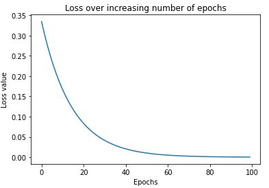
As you can see, the loss started at around 0.33 and steadily dropped to around 0.0001. This is an indication that weights are adjusted according to the input-output data and when an input is given, we can expect it to predict the output that we have been comparing it against in the loss function. The output weights are as follows:
[array([[ 0.01424004, -0.5907864 , -0.27549535],
        [ 0.39883757, -0.52918637, 0.18640439]], dtype=float32),
 array([ 0.00554004, 0.5519136 , -0.06599568], dtype=float32),
 array([[ 0.3475135 ],
        [-0.05529078],
        [ 0.03760847]], dtype=float32),
 array([-0.22443289], dtype=float32)]
- Once we have the updated weights, make the predictions for the input by passing the input through the network and calculate the output value:
pre_hidden = np.dot(x,W[0]) + W[1]
hidden = 1/(1+np.exp(-pre_hidden))
pred_out = np.dot(hidden, W[2]) + W[3]
# -0.017
The output of the preceding code is the value of -0.017, which is a value that is very close to the expected output of 0. As we train for more epochs, the pred_out value gets even closer to 0.
So far, we have learned about feedforward propagation and backpropagation. The key piece in the update_weights function that we defined here is the learning rate – which we will learn about in the next section.