Search icon
Arrow left icon
All Products
Best Sellers
New Releases
Books
Videos
Audiobooks
Learning Hub
Newsletters
Free Learning
Arrow right icon
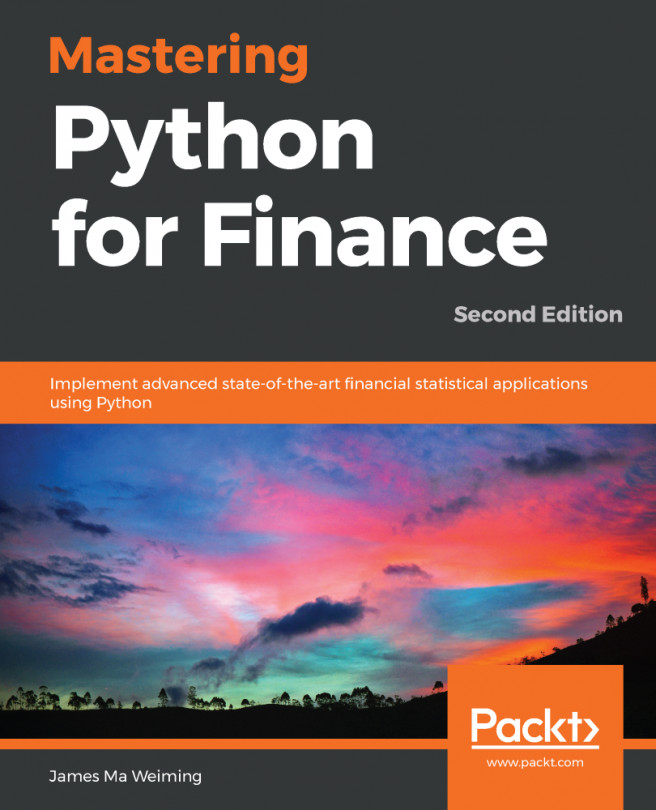
Mastering Python for Finance. - Second Edition

You're reading from  Mastering Python for Finance. - Second Edition

Product type Book
Published in Apr 2019
Publisher Packt
ISBN-13 9781789346466
Pages 426 pages
Edition 2nd Edition
Languages
Author (1):
James Ma Weiming James Ma Weiming
Profile icon James Ma Weiming

Table of Contents (16) Chapters

Preface Section 1: Getting Started with Python
Overview of Financial Analysis with Python Section 2: Financial Concepts
The Importance of Linearity in Finance Nonlinearity in Finance Numerical Methods for Pricing Options Modeling Interest Rates and Derivatives Statistical Analysis of Time Series Data Section 3: A Hands-On Approach
Interactive Financial Analytics with the VIX Building an Algorithmic Trading Platform Implementing a Backtesting System Machine Learning for Finance Deep Learning for Finance Other Books You May Enjoy

Modeling Interest Rates and Derivatives

Interest rates affect economic activities at all levels. Central banks, including the Federal Reserve (informally known as the Fed), target interest rates as a policy tool to influence economic activity. Interest rate derivatives are popular with investors who require customized cash flow needs or specific views on interest-rate movements.

One of the key challenges that interest-rate derivative traders face is to have a good and robust pricing procedure for these products. This involves understanding the complicated behavior of an individual interest-rate movement. Several interest-rate models have been proposed for financial studies. Some common models studied in finance are the Vasicek, CIR, and Hull-White models. These interest-rate models involve modeling the short-rate and rely on factors (or sources of uncertainty) with most of them...

Fixed-income securities

Corporations and governments issue fixed-income securities as a means of raising money. The owners of such debts lend money and expect to receive the principal when the debt matures. The issuer who wishes to borrow money may issue a fixed amount interest payment during the lifetime of the debt at pre-specified times.

The holders of debt securities, such as US Treasury bills, notes, and bonds, face the risk of default by the issuer. The federal government and municipal government are thought to face the least default risk, since they can easily raise taxes and create more money to repay the outstanding debts.

Most bonds pay a fixed amount of interest semi-annually, while some pay quarterly, or annually. These interest payments are also referred to as coupons. They are quoted as a percentage of the face value or par amount of the bond on an annual basis.

...

Yield curves

In a normal yield curve environment, long-term interest rates are higher than short-term interest rates. Investors expect to be compensated with higher returns when they lend money for a longer period since they are exposed to a higher default risk. The normal or positive yield curve is said to be upward sloping, as shown in the following graph:

In certain economic conditions, the yield curve can be inverted. Long-term interest rates are lower than short-term interest rates. Such a condition occurs when the supply of money is tight. Investors are willing to forgo long-term gains to preserve their wealth in the short-term. During periods of high inflation, where the inflation rate exceeds the rate of coupon interests, negative interest rates may be observed. Investors are willing to pay in the short-term just to secure their long-term wealth. The inverted yield curve...

Valuing a zero-coupon bond

A zero-coupon bond is a bond that does not pay any periodic interest except on maturity, where the principal or face value is repaid. Zero-coupon bonds are also called pure discount bonds.

A zero-coupon bond can be valued as follows:

Here, y is the annually-compounded yield or rate of the bond, and t is the time remaining to the maturity of the bond.

Let's take a look at an example of a five-year zero-coupon bond with a face value of $100. The yield is 5%, compounded annually. The price can be calculated as follows:

A simple Python zero-coupon bond calculator can be used to illustrate this example:

In [ ]:
def zero_coupon_bond(par, y, t):
"""
Price a zero coupon bond.

:param par: face value of the bond.
:param y: annual yield or rate of the bond.
:param t: time to maturity, in years.
...

Bootstrapping a yield curve

Short-term spot rates can be derived directly from various short-term securities, such as zero-coupon bonds, T-bills, notes, and eurodollar deposits. However, longer-term spot rates are typically derived from the prices of long-term bonds through a bootstrapping process, taking into account the spot rates of maturities that correspond to the coupon payment date. After obtaining short-term and long-term spot rates, the yield curve can then be constructed.

An example of bootstrapping the yield curve

Let's illustrate the bootstrapping of the yield curve with an example. The following table shows a list of bonds with different maturities and prices:

Bond face value in dollars

Time to maturity...

Forward rates

An investor who plans to invest at a later time may be curious to know what the future interest rate will look like, as implied by today's term structure of interest rates. For example, you might ask, What is the one-year spot rate one year from now? To answer this question, you can calculate forward rates for the period between T1 and T2 using this formula:

Here, r1 and r2 are the continuously-compounded annual interest rates at time periods T1 and T2, respectively.

The following ForwardRates class helps us generate a list of forward rates from a list of spot rates:

class ForwardRates(object):

def __init__(self):
self.forward_rates = []
self.spot_rates = dict()

def add_spot_rate(self, T, spot_rate):
self.spot_rates[T] = spot_rate

def get_forward_rates(self):
"""
Returns a list of forward rates
...

Calculating the yield to maturity

The yield to maturity (YTM) measures the interest rate, as implied by the bond, which takes into account the present value of all the future coupon payments and the principal. It is assumed that bond holders can invest received coupons at the YTM rate until the maturity of the bond; according to risk-neutral expectations, the payments received should be the same as the price paid for the bond.

Let's take a look at an example of a 5.75% bond that will mature in 1.5 years with a par value of 100. The price of the bond is $95.0428 and coupons are paid semi-annually. The pricing equation can be stated as follows:

Here:

  • c is the coupon dollar amount paid at each time period
  • T is the time period of payment in years
  • n is the coupon payment frequency
  • y is the YTM that we are interested in solving

To solve the YTM is typically a complex process...

Calculating the price of a bond

When the YTM is known, we can get back the bond price in the same way we used the pricing equation. This is implemented by the bond_price() function:

In [ ]:
def bond_price(par, T, ytm, coup, freq=2):
freq = float(freq)
periods = T*2
coupon = coup/100.*par
dt = [(i+1)/freq for i in range(int(periods))]
price = sum([coupon/freq/(1+ytm/freq)**(freq*t) for t in dt]) + \
par/(1+ytm/freq)**(freq*T)
return price

Plugging in the same values from the earlier example, we get the following result:

In [ ]:
price = bond_price(100, 1.5, ytm, 5.75, 2)
print(price)
Out[ ]:
95.04279999999997

This gives us the same original bond price discussed in the earlier example, Calculating the yield to maturity. With the bond_ytm() and bond_price() functions, we can apply these for further uses in bond pricing...

Bond duration

Duration is a sensitivity measure of bond prices to yield changes. Some duration measures are effective duration, Macaulay duration, and modified duration. The type of duration that we will discuss is modified duration, which measures the percentage change in bond price with respect to a percentage change in yield (typically 1% or 100 basis points (bps)).

The higher the duration of a bond, the more sensitive it is to yield changes. Conversely, the lower the duration of a bond, the less sensitive it is to yield changes.

The modified duration of a bond can be thought of as the first derivative of the relationship between price and yield:

Here:

  • dY is the given change in yield
  • P is the price of the bond from a decrease in yield by dY
  • P+ is the price of the bond from an increase in yield by dY
  • P0 is the initial price of the bond

It should be noted that the...

Bond convexity

Convexity is the sensitivity measure of the duration of a bond to yield changes. Think of convexity as the second derivative of the relationship between the price and yield:

Bond traders use convexity as a risk-management tool to measure the amount of market risk in their portfolio. Higher-convexity portfolios are less affected by interest-rate volatilities than lower-convexity portfolios, given the same bond duration and yield. As such, higher-convexity bonds are more expensive than lower-convexity ones, everything else being equal.

The implementation of a bond convexity is given as follows:

In [ ]:
def bond_convexity(price, par, T, coup, freq, dy=0.01):
ytm = bond_ytm(price, par, T, coup, freq)

ytm_minus = ytm - dy
price_minus = bond_price(par, T, ytm_minus, coup, freq)

ytm_plus = ytm + dy
price_plus = bond_price...

Short–rate modeling

In short-rate modeling, the short-rate, r(t), is the spot rate at a particular time. It is described as a continuously-compounded, annualized interest rate term for an infinitesimally short period of time on the yield curve. The short-rate takes on the form of a stochastic variable in interest-rate models, where the interest rates may change by small amounts at every point in time. Short-rate models attempt to model the evolution of interest rates over time, and hopefully describe the economic conditions at certain periods.

Short-rate models are frequently used in the evaluation of interest-rate derivatives. Bonds, credit instruments, mortgages, and loan products are sensitive to interest-rate changes. Short-rate models are used as interest rate components in conjunction with pricing implementations, such as numerical methods, to help price such derivatives...

Bond options

When bond issuers, such as corporations, issue bonds, one of the risks they face is the interest rate risk. When interest rates decrease, bond prices increase. While existing bondholders will find their bonds more valuable, bond issuers, on the other hand, find themselves in a losing position, since they will be issuing higher-interest payments than the prevailing interest rate. Conversely, when interest rates increase, bond issuers are at an advantage, since they are able to continue issuing the same low-interest payments as agreed to on the bond-contract specifications.

To capitalize on interest-rate changes, bond issuers may embed options within a bond. This allows the issuer the right, but not the obligation, to buy or sell the issued bond at a predetermined price during a specified period of time. An American type of bond option allows the issuer to exercise...

Pricing a callable bond option

In this section, we will take a look at pricing a callable bond. We assume that the bond to be priced is a zero-coupon paying bond with an embedded European call option. The price of a callable bond can be thought of as follows:

Price of callable bond = price of bond with no option − price of call option

Pricing a zero-coupon bond by the Vasicek model

The value of a zero-coupon bond with a par value of 1 at time t and a prevailing interest rate, r, is defined as follows:

Since the interest rate, r, is always changing, we rewrite the zero-coupon bond as follows:

Now, the interest rate, r, is a stochastic process that accounts for the price of the bond from time t to T, where T is the...

Summary

In this chapter, we focused on interest-rate and related derivative pricing with Python. Most bonds, such as US Treasury bonds, pay a fixed amount of interest semi-annually, while other bonds may pay quarterly or annually. It is a characteristic of bonds that their prices are closely related to current interest-rate levels in an inverse manner. The normal or positive yield curve, where long-term interest rates are higher than short-term interest rates, is said to be upward sloping. In certain economic conditions, the yield curve can be inverted and is said to be downward sloping.

A zero-coupon bond is a bond that pays no coupons during its lifetime, except upon maturity when the principal or face value is repaid. We implemented a simple zero-coupon bond calculator in Python.

The yield curve can be derived from the short-term zero or spot rates of securities, such as zero...

lock icon The rest of the chapter is locked
You have been reading a chapter from
Mastering Python for Finance. - Second Edition
Published in: Apr 2019 Publisher: Packt ISBN-13: 9781789346466
Register for a free Packt account to unlock a world of extra content!
A free Packt account unlocks extra newsletters, articles, discounted offers, and much more. Start advancing your knowledge today.
Unlock this book and the full library FREE for 7 days
Get unlimited access to 7000+ expert-authored eBooks and videos courses covering every tech area you can think of
Renews at $15.99/month. Cancel anytime}