Diagnosing Coronary Artery Disease

In this chapter, we will be predicting heart disease using neural networks. We will also be looking at a dataset from the UCI repository, which has data on 76 health-related attributes for over 300 patients. We will use this data to predict coronary artery disease. So, if you're looking to get started with machine learning in general—or, more specifically, machine learning applications in the field of healthcare; then this is the project for you.

In this chapter, we will familiarize ourselves with the following topics:

• The dataset
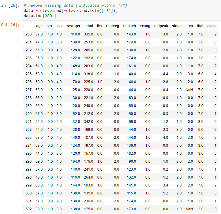
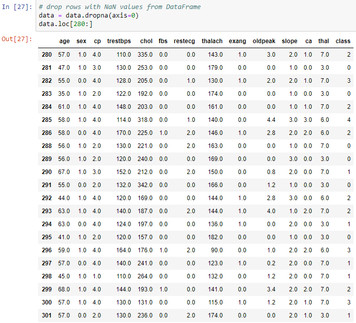
• Fixing missing data
• Splitting the dataset
• Training the neural network
• A comparison of categorical and binary problems

The dataset

To begin with, let's open Command Prompt and execute the following command:

cd tutorial
jupyter lab

This will take us to the tutorial folder. From here, we can open up JupyterLab. This folder is going to be empty right now, but it is where we will be completing this tutorial.

The dataset we're going to use is the heart disease dataset from the UCI repository. You can download this from archive.ics.uci.edu/ml/machine-learning-databases/heart-disease/. It has around 303 patients collected from the Cleveland Clinic Foundation. They have also added data from other places as well, but we are only going to look at data from Cleveland for now. If you go over to the Data folder, you'll see that we've got lot's of different options:

Even if you don't go to the preceding URL, we can directly import all of the files present there directly into our...

Fixing missing data

Fixing missing data in a dataset is the first important step for a lot of machine learning applications in healthcare, because we're often going to have missing data. There are different ways to handle this, and one of the easiest is to remove those rows entirely. This is especially the case if we're just trying to test a classification algorithm on a neural network, or train one for the first time. This is the route that we are going to take now:

We can see, from the data in our new DataFrame, that the question marks have been replaced with NaN. We have nothing in those particular locations. Consequently, we're going to drop the rows with NaN values (or non-number values) from the DataFrame, which is really easy to do with pandas:

In the preceding screenshot, we use the dropna() function to drop all the missing data. As we can see, the rows...

Splitting the dataset

Now we will split our dataset into training and testing datasets. We're going to use sklearn's train_test_split function to generate a training dataset, which will be about 80% of the total data, and then a testing dataset, which will be 20% of the total data. The class values in this dataset contain multiple types of heart disease, with values ranging from 0 (healthy) to 4 (severe heart disease). Consequently, we will convert our class data into categorical labels.

Let's create X and y datasets for training. So, first, we want to split our class label into its own y value. We will import the model_selection package from sklearn and convert the X DataFrame to a NumPy array, taking everything but the class attribute. Likewise, for the y DataFrame, we will convert this into a NumPy array, but here we will only take the class attribute. Then...

Training the neural network

Now, we will move on to building and training the neural network. To do so, let's import some specific layers from Keras. Then, we will define a create_model() function to build the Keras model, and define the model type as Sequential. After this, we will define an input layer, a hidden layer and an output layer, compile the model, and finally print the model:

As we see in the preceding screenshot, we have our model summary. We have 112 parameters for the first layer, 36 for the second, and 25 for the third layer. We have a total of 173 parameters. These are all trainable data for our neural network, which is what we will be using to classify the patients as either having coronary artery disease or not having coronary artery disease.

We will now fit the model to the training data using the model.fit() function:

From the preceding screenshot...

A comparison of categorical and binary problems

We will compare and contrast our categorical classification problem and the binary classification problem just covered. To do this, first we have to create a new model, since we've changed our data. We will define a binary model, then we will define an input layer, a hidden layer and an output layer, compile the model, and finally print the model:

As we see in the screenshot, our third layer has only one output value, so it's going to be 0 and 1, instead of a one-hot encoded vector for a categorical classification. So, our binary model is ready, and now we're in the training phase—let's fit the binary model to our binary data that we curated:

As we can see in the preceding screenshot, we're getting better accuracy than we were on our categorical classification problem. Binary classification is like...

Summary

In this chapter, we looked at how to use sklearn and Keras, how to import data from a UCI repository using the pandas read_csv function, and how to preprocess that data. One of the ways to handle missing data, whether in healthcare applications or not, is to remove the rows or instances that have missing attributes. We then learned how to describe the data and print out histograms so we know what we're working with, followed by doing a train/test split with model_selection from sklearn. Furthermore, we also learned how to convert one-hot encoded vectors for a categorical classification, by defining simple neural networks using Keras. We then looked at types of activation function, such as softmax, for categorical classifications with categorical_crossentropy. In contrast, when we got to our binary classification, we used a sigmoid activation function and a binary_crossentropy...