Chapter 3. Data Exploration

When we first receive a dataset, most of the times we only know what it is related to—an overview that is not enough to start applying algorithms or create models on it. Data exploration is of paramount importance in data science. It is the necessary process prior to creating a model because it gives a highlight of the dataset and definitely makes clear the path to achieving our objectives. Data exploration familiarizes the data scientist with the data and helps to know what general hypothesis we can infer from the dataset. So, we can say it is a process of extracting some information from the dataset, not knowing beforehand what to look for.

In this chapter, we will study:

• Sampling, population, and weight vectors

• Inferring column types

• Summary of a dataset

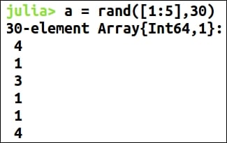
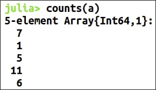
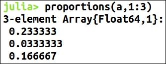
• Scalar statistics

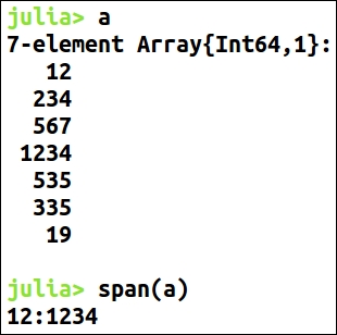
• Measures of variation

• Data exploration using visualizations

Data exploration involves descriptive statistics. Descriptive statistics is a field of data analysis that finds out patterns by meaningfully...

Sampling

In the previous example, we spoke about calculating the mean height of 1,000 people out of the 10 million people living in New Delhi. While gathering the data of these 10 million people, let's say we started from a particular age or community, or in any sequential manner. Now, if we take 1,000 people who are consecutive in the dataset, there is a high probability that they would have similarities among them. This similarity would not give us the actual highlight of the dataset that we are trying to achieve. So, taking a small chunk of consecutive data points from the dataset wouldn't give us the insight that we want to gain. To overcome this, we use sampling.

Sampling is a technique to randomly select data from the given dataset such that they are not related to each other, and therefore we can generalize the results that we generate on this selected data over the complete dataset. Sampling is done over a population.

Population

A population in statistics refers to the set of all the...

Inferring column types

To understand the dataset and move any further, we need to first understand what type of data we have. As our data is stored in columns, we should know their type before performing any operations. This is also called creating a data dictionary:

julia> typeof(iris_dataframe[1,:SepalLength]) 
Float64 
 
julia> typeof(iris_dataframe[1,:Species]) 
ASCIIString 

We have used the classic dataset of iris here. We already know the type of the data in these columns. We can apply the same function to any similar dataset. Suppose we were only given columns without labels; then it would have been hard to determine the type of data these columns contain. Sometimes, the dataset looks as if it contains numeric digits but their data type is ASCIIString. These can lead to errors in further steps. These errors are avoidable.

Basic statistical summaries

Although, we are currently using RDatasets, about which we have sufficient details and documentation, these methods and techniques can be extended to other datasets.

Let's use a different dataset:

We are using another dataset from the RDatasets package. These are exam scores from Inner London. To get some information about the dataset, we will use the describe() function, which we have already discussed in previous chapters:

The columns are described as follows:

• Length refers to the number of records (rows).

• Type refers to the data type of the column. Therefore, School is of the Pooled ASCIIString data type.

• NA and NA% refer to the number and percentage of the NA values present in the column. This is really helpful as you don't need to manually check for missing records now.

• Unique refers to the number of unique records present in the column.

• Min and Max are the minimum and maximum values present in the column (this does not apply to columns having ASCIIStrings...

Scalar statistics

Various functions are provided by Julia's package to compute various statistics. These functions are used to describe data in different ways as required.

Standard deviations and variances

The mean and median we earlier computed (in the describe() function) are measures of central tendency. Mean refers to the center computed after applying weights to all the values and median refers to the center of the list.

This is only one piece of information and we would like to know more about the dataset. It would be good to have knowledge about the spread of data points across the dataset. We cannot use just the min and max functions as we can have outliers in the dataset. Therefore, these min and max functions will lead to incorrect results.

Variance is a measurement of the spread between data points in a dataset. It is computed by calculating the distance of numbers from the mean. Variance measures how far each number in the set is from the mean.

The following is the formula for variance...

Measures of variation

It is good to have knowledge of the variation of values in the dataset. Various statistical functions facilitate:

• span(arr): span is used to calculate the total spread of the dataset, which is maximum(arr) to minimum(arr):

• variation(arr): Also called the coefficient of variance. It is the ratio of the standard deviation to the mean of the dataset. In relation to the mean of the population, CV denotes the extent of variability. Its advantage is that it is a dimensionless number and can be used to compare different datasets.

Standard error of mean: We work on different samples drawn from the population. We compute the means of these samples and call them sample means. For different samples, we wouldn't be having the same sample mean but a distribution of sample means. The standard deviation of the distribution of these sample means is called standard error of mean.

In Julia, we can compute standard error of mean using sem(arr).

Mean absolute deviation is a robust measure...

Scatter matrix and covariance

Covariance is used very often by data scientists to find out how two ordered sets of data follow in the same direction. It can very easily define whether the variables are correlated or not. To best represent this behavior, we create a covariance matrix. The unnormalized version of the covariance matrix is the scatter matrix.

To create a scatter matrix, we use the scattermat(arr) function.

The default behavior is to treat each row as an observation and column as a variable. This can be changed by providing the keyword arguments vardim and mean:

• Vardim: vardim=1 (default) means each column is a variable and each row is an observation. vardim=2 is the reverse.

• mean: The mean is computed by scattermat. We can use a predefined mean to save compute cycles.

We can also create a weighted covariance matrix using the cov function. It also takes vardim and mean as optional arguments for the same purpose.

Computing deviations

StatsBase.jl provides various functions to compute deviations between two datasets. This can be calculated using other functions, but to facilitate and for ease of use, StatsBase provides these efficiently implemented functions:

• Mean absolute deviation: For two datasets, a and b, it is calculated as meanad(x,y) which is a wrapper over mean(abs(x-y)).

• Maximum absolute deviation: For two datasets, a and b, it is calculated as maxad(x,y), which is a wrapper over maximum(abs(x-y)).

• Mean squared deviation: For two datasets, a and b, it is calculated as msd(x,y), which is a wrapper over mean(abs2(x-y)).

• Root mean squared deviation: For two datasets, a and b, it is calculated as rmsd(a,b), which is a wrapper over sqrt(msd(a, b)).

Rankings

When a dataset is sorted in ascending order, a rank is assigned to each value. Ranking is a process where the dataset is transformed and values are replaced by their ranks. Julia provides functions for various types of rankings.

In ordinal ranking, all items in the dataset are assigned a distinct value. Items that have equal values are assigned a ranking arbitrarily. In Julia, this is done using the ordinalrank function.

Suppose this is our dataset and we want to do ordinal ranking:

Using the ordinalrank(arr) function, we've got the ordinal ranking. Similarly, StatsBase also provides functions to find other types of rankings, such as competerank(), denserank(), and tiedrank().

Counting functions

In data exploration, counting over a range is often done. It helps to find out the most/least occurring value. Julia provides the counts function to count over a range. Let's say we have an array of values. For our convenience, we will now use the random function to create an array:

We have created an array of 30 values ranging from 1 to 5. Now we want to know how many times they occur in the dataset:

Using the count function, we found that 1(7), 2(1), 3(5), 4(11), and 5(6). counts take different arguments to suit the use case.

The proportions() function is used to compute the proportions of the values in the dataset and  Julia provides the function:

We calculated proportions on the same dataset that we used in the previous examples. It shows that the ratio of value 1 in the dataset is 0.23333. This can also be seen as the probability of finding the value in the dataset.

Other count functions include:

• countmap(arr): This is a map function that maps the values to the number...

Histograms

Data exploration after a basic understanding can also be done with the aid of visualizations. Plotting a histogram is one of the most common ways of data exploration through visualization. A histogram type is used to tabulate data over a real plane separated into regular intervals.

A histogram is created using the fit method:

julia> fit(Histogram, data[, weight][, edges])  

fit takes the following arguments:

• data: Data is passed to the fit function in the form of a vector, which can either be one-dimensional or n-dimensional (tuple of vectors of equal length).

• weight: This is the optional argument. A WeightVec type can be passed as an argument if values have different weights. The default weight of values is 1.

• edges: This is a vector used to give the edges of the bins along each dimension.

It also takes a keyword argument, nbins, which is used to define the number of bins that the histogram should use along each side:

In this example, we used two random value generators...

Correlation analysis

Julia provides some functions to facilitate correlation analysis. Correlation and dependence are two common terms in statistics. Dependence refers to one variable having a statistical relationship with another variable, whereas correlation is one variable having a much wider class of relationship with the other variable, which may also include dependence.

The autocov(x) function is used to compute auto-covariance of x. It returns a vector of the same size as x.

This is a dataset we generated. We can apply autocov on this dataset:

To compute auto-correlation, we use the autocor function:

Similarly, we can also compute cross-covariance and cross-correlation. For that, we will generate another random array of the same size:

Cross-covariance and cross-correlation of 2 arrays of length=6 results in arrays of lengths=11.

Summary

In this chapter, we discussed why data exploration is important and how can we perform exploratory analysis on datasets.

These are the various important techniques and concepts that we discussed:

• Sampling is a technique to randomly select unrelated data from the given dataset so that we can generalize the results that we generate on this selected data over the complete dataset.

• Weight vectors are important when the dataset that we have or gather doesn't represent the actual data.

• Why it is necessary to know the column types and how summary functions can be really helpful in getting the gist of the dataset.

• Mean, median, mode, standard deviation, variance, and scalar statistics, and how they are implemented in Julia.

• Measuring the variations in a dataset is really important and z-scores and entropy can be really useful.

• After some basic data cleaning and some understanding, visualization can be very beneficial and insightful.

References

• http://julia.readthedocs.io/en/latest/manual/

• https://dataframesjl.readthedocs.io/en/latest/

• https://github.com/JuliaStats/StatsBase.jl

• http://dcjones.github.io/Gadfly.jl/