Handling Data with pandas DataFrame
The pandas library is an extremely resourceful open source toolkit for handling, manipulating, and analyzing structured data. Data tables can be stored in the DataFrame object available in pandas, and data in multiple formats (for example, .csv, .tsv, .xlsx, and .json) can be read directly into a DataFrame. Utilizing built-in functions, DataFrames can be efficiently manipulated (for example, converting tables between different views, such as, long/wide; grouping by a specific column/feature; summarizing data; and more).
Reading Data from Files
Most small-to medium-sized datasets are usually available or shared as delimited files such as comma-separated values (CSV), tab-separated values (TSV), Excel (.xslx), and JSON files. Pandas provides built-in I/O functions to read files in several formats, such as, read_csv, read_excel, and read_json, and so on into a DataFrame. In this section, we will use the diamonds dataset (hosted in book GitHub repository).
Note
The datasets used here can be found in https://github.com/TrainingByPackt/Interactive-Data-Visualization-with-Python/tree/master/datasets.
Exercise 1: Reading Data from Files
In this exercise, we will read from a dataset. The example here uses the diamonds dataset:
- Open a jupyter notebook and load the
pandasandseabornlibraries:#Load pandas library import pandas as pd import seaborn as sns
- Specify the URL of the dataset:
#URL of the dataset
diamonds_url = "https://raw.githubusercontent.com/TrainingByPackt/Interactive-Data-Visualization-with-Python/master/datasets/diamonds.csv"
- Read files from the URL into the
pandasDataFrame:#Yes, we can read files from a URL straight into a pandas DataFrame! diamonds_df = pd.read_csv(diamonds_url) # Since the dataset is available in seaborn, we can alternatively read it in using the following line of code diamonds_df = sns.load_dataset('diamonds')The dataset is read directly from the URL!
Note
Use the
usecolsparameter if only specific columns need to be read.
The syntax can be followed for other datatypes using, as shown here:
diamonds_df_specific_cols = pd.read_csv(diamonds_url, usecols=['carat','cut','color','clarity'])
Observing and Describing Data
Now that we know how to read from a dataset, let's go ahead with observing and describing data from a dataset. pandas also offers a way to view the first few rows in a DataFrame using the head() function. By default, it shows 5 rows. To adjust that, we can use the argument n—for instance, head(n=5).
Exercise 2: Observing and Describing Data
In this exercise, we'll see how to observe and describe data in a DataFrame. We'll be again using the diamonds dataset:
- Load the
pandasandseabornlibraries:#Load pandas library import pandas as pd import seaborn as sns
- Specify the URL of the dataset:
#URL of the dataset
diamonds_url = "https://raw.githubusercontent.com/TrainingByPackt/Interactive-Data-Visualization-with-Python/master/datasets/diamonds.csv"
- Read files from the URL into the
pandasDataFrame:#Yes, we can read files from a URL straight into a pandas DataFrame! diamonds_df = pd.read_csv(diamonds_url) # Since the dataset is available in seaborn, we can alternatively read it in using the following line of code diamonds_df = sns.load_dataset('diamonds') - Observe the data by using the
headfunction:diamonds_df.head()
The output is as follows:

Figure 1.1: Displaying the diamonds dataset
The data contains different features of diamonds, such as
carat,cutquality,color, andprice, as columns. Now,cut,clarity, andcolorare categorical variables, andx,y,z,depth,table, andpriceare continuous variables. While categorical variables take unique categories/names as values, continuous values take real numbers as values.cut,color, andclarityare ordinal variables with5,7, and8unique values (can be obtained bydiamonds_df.cut.nunique(),diamonds_df.color.nunique(),diamonds_df.clarity.nunique()– try it!), respectively.cutis the quality of the cut, described asFair,Good,Very Good,Premium, orIdeal;colordescribes the diamond color fromJ (worst)toD (best). There's alsoclarity, which measures how clear the diamond is—the degrees areI1 (worst),SI1,SI2,VS1,VS2,VVS1,VVS2, andIF (best). - Count the number of rows and columns in the DataFrame using the
shapefunction:diamonds_df.shape
The output is as follows:
(53940, 10)
The first number,
53940, denotes the number of rows and the second,10, denotes the number of columns. - Summarize the columns using
describe()to obtain the distribution of variables, includingmean,median,min,max, and the different quartiles:diamonds_df.describe()
The output is as follows:

Figure 1.2: Using the describe function to show continuous variables
This works for continuous variables. However, for categorical variables, we need to use the
include=objectparameter. - Use
include=objectinside thedescribefunction for categorical variables (cut,color,clarity):diamonds_df.describe(include=object)
The output is as follows:

Figure 1.3: Use the describe function to show categorical variables
Now, what if you would want to see the column types and how much memory a DataFrame occupies?
- To obtain information on the dataset, use the
info()method:diamonds_df.info()
The output is as follows:
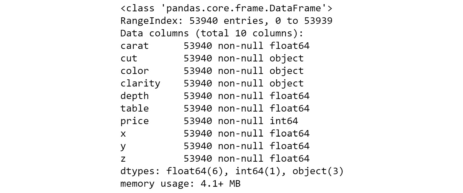
Figure 1.4: Information on the diamonds dataset
The preceding figure shows the data type (float64, object, int64..) of each of the columns, and memory (4.1MB) that the DataFrame occupies. It also tells the number of rows (53940) present in the DataFrame.
Selecting Columns from a DataFrame
Let's see how to select specific columns from a dataset. A column in a pandas DataFrame can be accessed in two simple ways: with the . operator or the [ ] operator. For example, we can access the cut column of the diamonds_df DataFrame with diamonds_df.cut or diamonds_df['cut']. However, there are some scenarios where the . operator cannot be used:
- When the column name contains spaces
- When the column name is an integer
- When creating a new column
Now, how about selecting all rows corresponding to diamonds that have the Ideal cut and storing them in a separate DataFrame? We can select them using the loc functionality:
diamonds_low_df = diamonds_df.loc[diamonds_df['cut']=='Ideal']
diamonds_low_df.head()
The output is as follows:
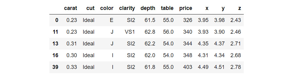
Figure 1.5: Selecting specific columns from a DataFrame
Here, we obtain indices of rows that meet the criterion:
[diamonds_df['cut']=='Ideal' and then select them using loc.
Adding New Columns to a DataFrame
Now, we'll see how to add new columns to a DataFrame. We can add a column, such as, price_per_carat, in the diamonds DataFrame. We can divide the values of two columns and populate the data fields of the newly added column.
Exercise 3: Adding New Columns to the DataFrame
In this exercise, we are going to add new columns to the diamonds dataset in the pandas library. We'll start with the simple addition of columns and then move ahead and look into the conditional addition of columns. To do so, let's go through the following steps:
- Load the
pandasandseabornlibraries:#Load pandas library import pandas as pd import seaborn as sns
- Specify the URL of the dataset:
#URL of the dataset
diamonds_url = "https://raw.githubusercontent.com/TrainingByPackt/Interactive-Data-Visualization-with-Python/master/datasets/diamonds.csv"
- Read files from the URL into the
pandasDataFrame:#Yes, we can read files from a URL straight into a pandas DataFrame! diamonds_df = pd.read_csv(diamonds_url) # Since the dataset is available in seaborn, we can alternatively read it in using the following line of code diamonds_df = sns.load_dataset('diamonds')Let's look at simple addition of columns.
- Add a
price_per_caratcolumn to the DataFrame:diamonds_df['price_per_carat'] = diamonds_df['price']/diamonds_df['carat']
- Call the DataFrame
headfunction to check whether the new column was added as expected:diamonds_df.head()
The output is as follows:

Figure 1.6: Simple addition of columns
Similarly, we can also use addition, subtraction, and other mathematical operators on two numeric columns.
Now, we'll look at conditional addition of columns. Let's try and add a column based on the value in
price_per_carat, say anything more than3500as high (coded as1) and anything less than3500as low (coded as0). - Use the
np.wherefunction from Python'snumpypackage:#Import numpy package for linear algebra import numpy as np diamonds_df['price_per_carat_is_high'] = np.where(diamonds_df['price_per_carat']>3500,1,0) diamonds_df.head()
The output is as follows:
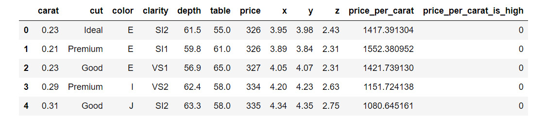
Figure 1.7: Conditional addition of columns
Therefore, we have successfully added two new columns to the dataset.
Applying Functions on DataFrame Columns
You can apply simple functions on a DataFrame column—such as, addition, subtraction, multiplication, division, squaring, raising to an exponent, and so on. It is also possible to apply more complex functions on single and multiple columns in a pandas DataFrame. As an example, let's say we want to round off the price of diamonds to its ceil (nearest integer equal to or higher than the actual price). Let's explore this through an exercise.
Exercise 4: Applying Functions on DataFrame columns
In this exercise, we'll consider a scenario where the price of diamonds has increased and we want to apply an increment factor of 1.3 to the price of all the diamonds in our record. We can achieve this by applying a simple function. Next, we'll round off the price of diamonds to its ceil. We'll achieve that by applying a complex function.Let's go through the following steps:
- Load the
pandasandseabornlibraries:#Load pandas library import pandas as pd import seaborn as sns
- Specify the URL of the dataset:
#URL of the dataset
diamonds_url = "https://raw.githubusercontent.com/TrainingByPackt/Interactive-Data-Visualization-with-Python/master/datasets/diamonds.csv"
- Read files from the URL into the
pandasDataFrame:#Yes, we can read files from a URL straight into a pandas DataFrame! diamonds_df = pd.read_csv(diamonds_url) # Since the dataset is available in seaborn, we can alternatively read it in using the following line of code diamonds_df = sns.load_dataset('diamonds') - Add a
price_per_caratcolumn to the DataFrame:diamonds_df['price_per_carat'] = diamonds_df['price']/diamonds_df['carat']
- Use the
np.wherefunction from Python'snumpypackage:#Import numpy package for linear algebra import numpy as np diamonds_df['price_per_carat_is_high'] = np.where(diamonds_df['price_per_carat']>3500,1,0)
- Apply a simple function on the columns using the following code:
diamonds_df['price']= diamonds_df['price']*1.3
- Apply a complex function to round off the price of diamonds to its ceil:
import math
diamonds_df['rounded_price']=diamonds_df['price'].apply(math.ceil)
diamonds_df.head()
The output is as follows:

Figure 1.8: Dataset after applying simple and complex functions
In this case, the function we wanted for rounding off to the ceil was already present in an existing library. However, there might be times when you have to write your own function to perform the task you want to accomplish. In the case of small functions, you can also use the
lambdaoperator, which acts as a one-liner function taking an argument. For example, say you want to add another column to the DataFrame indicating the rounded-off price of the diamonds to the nearest multiple of100(equal to or higher than the price). - Use the
lambdafunction as follows to round off the price of the diamonds to the nearest multiple of100:import math diamonds_df['rounded_price_to_100multiple']=diamonds_df['price'].apply(lambda x: math.ceil(x/100)*100) diamonds_df.head()
The output is as follows:

Figure 1.9: Dataset after applying the lambda function
Of book, not all functions can be written as one-liners and it is important to know how to include user-defined functions in the
applyfunction. Let's write the same code with a user-defined function for illustration. - Write code to create a user-defined function to round off the price of the diamonds to the nearest multiple of
100:import math def get_100_multiple_ceil(x): y = math.ceil(x/100)*100 return y diamonds_df['rounded_price_to_100multiple']=diamonds_df['price'].apply(get_100_multiple_ceil) diamonds_df.head()
The output is as follows:

Figure 1.10: Dataset after applying a user-defined function
Interesting! Now, we had created an user-defined function to add a column to the dataset.
Exercise 5: Applying Functions on Multiple Columns
When applying a function on multiple columns of a DataFrame, we can similarly use lambda or user-defined functions. We will continue to use the diamonds dataset. Suppose we are interested in buying diamonds that have an Ideal cut and a color of D (entirely colorless). This exercise is for adding a new column, desired to the DataFrame, whose value will be yes if our criteria are satisfied and no if not satisfied. Let's see how we do it:
- Import the necessary modules:
import seaborn as sns
import pandas as pd
- Import the
diamondsdataset fromseaborn:diamonds_df_exercise = sns.load_dataset('diamonds') - Write a function to determine whether a record,
x, is desired or not:def is_desired(x): bool_var = 'yes' if (x['cut']=='Ideal' and x['color']=='D') else 'no' return bool_var
- Use the
applyfunction to add the new column,desired:diamonds_df_exercise['desired']=diamonds_df_exercise.apply(is_desired, axis=1) diamonds_df_exercise.head()
The output is as follows:

Figure 1.11: Dataset after applying the function on multiple columns
The new column desired is added!
Deleting Columns from a DataFrame
Finally, let's see how to delete columns from a pandas DataFrame. For example, we will delete the rounded_price and rounded_price_to_100multiple columns. Let's go through the following exercise.
Exercise 6: Deleting Columns from a DataFrame
In this exercise, we will delete columns from a pandas DataFrame. Here, we'll be using the diamonds dataset:
- Import the necessary modules:
import seaborn as sns
import pandas as pd
- Import the
diamondsdataset fromseaborn:diamonds_df = sns.load_dataset('diamonds') - Add a
price_per_caratcolumn to the DataFrame:diamonds_df['price_per_carat'] = diamonds_df['price']/diamonds_df['carat']
- Use the
np.wherefunction from Python'snumpypackage:#Import numpy package for linear algebra import numpy as np diamonds_df['price_per_carat_is_high'] = np.where(diamonds_df['price_per_carat']>3500,1,0)
- Apply a complex function to round off the price of diamonds to its ceil:
import math
diamonds_df['rounded_price']=diamonds_df['price'].apply(math.ceil)
- Write a code to create a user-defined function:
import math
def get_100_multiple_ceil(x):
    y = math.ceil(x/100)*100
    return y

diamonds_df['rounded_price_to_100multiple']=diamonds_df['price'].apply(get_100_multiple_ceil)
- Delete the
rounded_priceandrounded_price_to_100multiplecolumns using thedropfunction:diamonds_df=diamonds_df.drop(columns=['rounded_price', 'rounded_price_to_100multiple']) diamonds_df.head()
The output is as follows:

Figure 1.12: Dataset after deleting columns
Note
By default, when the apply or drop function is used on a pandas DataFrame, the original DataFrame is not modified. Rather, a copy of the DataFrame post modifications is returned by the functions. Therefore, you should assign the returned value back to the variable containing the DataFrame (for example, diamonds_df=diamonds_df.drop(columns=['rounded_price', 'rounded_price_to_100multiple'])).
In the case of the drop function, there is also a provision to avoid assignment by setting an inplace=True parameter, wherein the function performs the column deletion on the original DataFrame and does not return anything.
Writing a DataFrame to a File
The last thing to do is write a DataFrame to a file. We will be using the to_csv() function. The output is usually a .csv file that will include column and row headers. Let's see how to write our DataFrame to a .csv file.
Exercise 7: Writing a DataFrame to a File
In this exercise, we will write a diamonds DataFrame to a .csv file. To do so, we'll be using the following code:
- Import the necessary modules:
import seaborn as sns
import pandas as pd
- Load the
diamondsdataset fromseaborn:diamonds_df = sns.load_dataset('diamonds') - Write the diamonds dataset into a .csv file:
diamonds_df.to_csv('diamonds_modified.csv') - Let's look at the first few rows of the DataFrame:
print(diamonds_df.head())
The output is as follows:

Figure 1.13: The generated .csv file in the source folder
By default, the
to_csvfunction outputs a file that includes column headers as well as row numbers. Generally, the row numbers are not desirable, and anindexparameter is used to exclude them: - Add a parameter
index=Falseto exclude the row numbers:diamonds_df.to_csv('diamonds_modified.csv', index=False)
And that's it! You can find this .csv file in the source directory. You are now equipped to perform all the basic functions on pandas DataFrames required to get started with data visualization in Python.
In order to prepare the ground for using various visualization techniques, we went through the following aspects of handling pandas DataFrames:
- Reading data from files using the
read_csv( ),read_excel( ), andreadjson( )functions - Observing and describing data using the
dataframe.head( ),dataframe.tail( ),dataframe.describe( ), anddataframe.info( )functions - Selecting columns using the
dataframe.column__nameordataframe['column__name']notation - Adding new columns using the
dataframe['newcolumnname']=...notation - Applying functions to existing columns using the
dataframe.apply(func)function - Deleting columns from DataFrames using the
_dataframe.drop(column_list)function - Writing DataFrames to files using the
_dataframe.tocsv()function
These functions are useful for preparing data in a format suitable for input to visualization functions in Python libraries such as seaborn.