Continuous-time Markov chains are quite similar to discrete-time Markov chains except for the fact that in the continuous case we explicitly model the transition time between the states using a positive-value random variable. Also, we consider the system at all possible values of time instead of just the transition times.
Continuous-time Markov chains
Exponential distributions
The random variable x is said to have an exponential distribution with a rate of distribution of λ if its probability density function is defined as follows:

Here, the rate of distribution λ needs to be greater than 0. We can also compute the expectation of X as this:

We see that the expectation of X is inversely proportional to the rate of learning. This means that an exponential distribution with a higher rate of learning would have a lower expectation. The exponential distribution is often used to model problems that involve modelling time until some event happens. A simple example could be modelling the time before an alarm clock goes off, or the time before a server comes to your table in a restaurant. And, as we know  , the higher the learning rate, the sooner we would expect the event to happen, and hence the name learning rate.
We can also compute the second moment and the variance of the exponential distribution:

And, using the first moment and the second moment, we can compute the variance of the distribution:

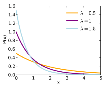
Figure 1.x: Probability distribution of exponential distribution


Now we will move on to some of the properties of the exponential distribution that are relevant to our example:
- Memoryless: Figure 1.x shows a plot of an exponential distribution. In the diagram, we can clearly see that the graph after any given point (a in this case) is an exact copy of the original distribution. We can also say that an exponential distribution that is conditioned on (X > a) still stays exponential. If we think about this property in terms of our examples, it means that if we had an alarm clock, and at any time, t, we check that it still hasn't gone off, we can still determine the distribution over the time ahead of t, which will be the same exponential distribution. This property of the exponential distribution is known as being memoryless, since at any given point in time, if you know the current state of the system (in this example, that the alarm hasn't gone off), you can determine the probability distribution over time in the future. This property of exponential distributions is quite similar to Markov chains, as you may recall from previous sections.
- Probability of minimum value: Let's say we have n independent exponential distributions over the random variables X0, . . ., Xn with learning rates λ0, ..., λn, respectively. For these distributions, we can prove that the distribution of min(X0, . . ., Xn) is also an exponential distribution with learning rate
 :
:

We will use both of these properties of the exponential distribution in our example for the continuous time Markov chain in a later section.
Poisson process
The Poisson process is a continuous process, and there can be multiple interpretations of it, which lead to different possible definitions. In this section, we will start with the formal definition and build up to a more simple, intuitive definition. A continuous-time stochastic process N(t):t > 0 is a Poisson process with a rate λ > 0 if the following conditions are met:
- N(0) = 0
- It has stationary and independent increments
- The distribution of N(t) is Poisson with mean λt:

First of all, we need to define what the stationary and independent increments are. For a continuous-time stochastic process, X(t): ≥ 0, an increment is defined as the difference in state of the system between two time instances; that is, given two time instances s and t with s < t, the increment from time s to time t is X(t) - X(s). As the name suggests, a process is said to have a stationary increment if its distribution for the increment depends only on the time difference.
In other words, a process is said to have a stationary increment if the distribution of X(t1) - X(s1) is equal to X(t2) - X(s2) if t1 > s1,t2 > s2 and t1 - s1 = t2 -s2. A process is said to have an independent increment if any two increments in disjointed time intervals are independent; that is, if t1 > s1 > t2 > s2, then the increments X(t2) - X(s2) and X(t1) - X(s1) are independent.
Now let's come back to defining the Poisson process. The Poisson process is essentially a counting process that counts the number of events that have occurred before time t. This count of the number of events before time t is given by N(t), and, similarly, the number of events occurring between time intervals t and t + s is given by N(t + s) - N(t). The value N(t + s) - N(t) is Poisson-distributed with a mean λs. We can see that the Poisson process has stationary increments in fixed time intervals, but as  , the value of N(t) will also approach infinity; that is,
  . Another thing worth noting is that, as the value of λ increases, the number of events happening will also increase, and that is why λ is also known as the rate of the process.
This brings us to our second simplified definition of the Poisson process. A continuous-time stochastic process N(t): t ≥ 0 is called a Poisson process with the rate of learning λ > 0 if the following conditions are met:
- N(0) = 0
- It is a counting process; that is, N(T) gives the count of the number of events that have occurred before time t
- The times between the events are distributed independently and identically, with an exponential distribution having a learning rate of λ
Continuous-time Markov chain example
Now, since we have a basic understanding of exponential distributions and the Poisson process, we can move on to the example to build up a continuous-time Markov chain. In this example, we will try to show how the properties of exponential distributions can be used to build up generic continuous-time Markov chains. Let's consider a hotel reception where n receptionists are working in parallel. Also consider that the guests arrive according to a Poisson process, with rate λ, and the service time for each guest is represented using an exponential random variable with learning rate µ. Also, if all the receptionists are busy when a new guest arrives, he/she will depart without getting any service. Now let's consider that a new guest arrives and finds all the receptionists are busy, and let's try to compute the expected number of busy receptionists in the next time interval.
Let's start by assuming that Tk represents the number of k busy receptionists in the next time instance. We can also use Tk to represent the expected number of busy receptionists found by the next arriving guest if k receptionists are busy at the current time instance. These two representations of Tk are equivalent because of the memoryless property of exponential distributions.
Firstly, T0 is clearly 0, because if there are currently 0 busy receptionists, the next arrival will also find 0 busy receptionists for sure. Now, considering T1, if there are currently i busy receptionists, the next arriving guest will find 1 busy receptionist if the time to the next arrival is less than the remaining service time for the busy receptionist. From the memoryless property, we know that the next arrival time is exponentially distributed with a learning rate of λ, and the remaining service time is also exponentially distributed with a learning rate of µ. Therefore, the probability that the next guest will find one receptionist busy is  and hence the following is true:

In general, we consider the situation that k receptionists are busy. We can obtain an expression for Tk by conditioning on what happens first. When we have k receptionists busy, we can think of basically k+1 independent exponential distributions: k exponentials with a learning rate of µ for the remaining service time for each receptionist, and 1 exponential distribution with a learning rate of λ for the next arriving guest. In our case, we want to condition on whether a service completion happens first or a new guest arrives first. The time for a service completion will be the minimum of the k exponentials. This first completion time is also exponentially distributed with a learning rate of kµ. Now, the probability of having a service completion before the next guest arrives is  . Similarly, the probability of the next thing happening being a guest arrival is
  .
.
Now, based on this, we can say that if the next event is service completion, then the expected number of busy receptionists will be Tk-1. Otherwise, if a guest arrives first, there will be k busy receptionists. Therefore we have the following:

We need to just solve this recursion now. T2 will be given by this equation:

If we continue this same pattern, we will get T3 as follows:

We can see a pattern in the values of T1 and T2, and therefore we can write a general term for it as follows:

Let's point out our observations on the previous example:
- At any given time instance, if there are i busy receptionists, for i < n there are i + 1 independent exponential distributions, with i of them having rate µ, and 1 of them having rate λ. The time until the process makes a jump is exponential, and its rate is given by iµ + λ. If all the receptionists are busy, then only the n exponential distributions corresponding to the service time can trigger a jump, and the time until the process makes a jump is exponential with rate nµ.
- When the process jumps from state i, for i < n, it jumps to state i + 1 with probability
 , and jumps to state i - 1 with probability of
  .
. - When the process makes a jump from state i, we can start up a whole new set of distributions corresponding to the state we jumped to. This is because, even though some of the old exponential distributions haven't triggered, it's equivalent to resetting or replacing those distributions.
Every time we jump to state i, regardless of when the time is, the distribution of how long we stay in state i and the probabilities of where we jump to next when we leave state i are the same. In other words, the process is time-homogeneous.
The preceding description of a continuous-time stochastic process corresponds to a continuous-time Markov chain. In the next section, we will try to define it in a more formal way.
Continuous-time Markov chain
In the previous section, we showed an example of a continuous-time Markov chain to give an indication of how it works. Let's now move on to formally define it. In a continuous-time Markov chain with a discrete state space S, for each state i ∈ S we have an associated set of ni independent exponential distributions with rates qi, j1, ..., qi,jni, where j1, ..., jni is the set of possible states the process may jump to when it leaves state i. And, when the process enters state i, the amount of time it spends in state i is exponentially distributed with rate vi = qij1+...+qijni, and when it leaves state i it will go to state jl with probability  for l = 1, ...,ni.
We can also extend the Markov property from the discrete-time case to continuous time.
For a continuous-time stochastic process (X(t) : t ≥ 0) with state space S, we say it has the Markov property if the following condition is met:

Here, 0 ≤ t1 ≤ t2 ≤. . . .tn-1 ≤ s ≤ t is any non-decreasing sequence of n + 1 times, and i1, i2, . . ., in-1, i, j ∈ S are any n + 1 states in the state space, for any integer n ≥ 1.
Similarly, we can extend time-homogeneity to the case of continuous-time Markov chains. We say that a continuous-time Markov chain is time homogenous if, for any s ≤ t, and any states i, j ∈ S, the following condition is met:

As in the case of discrete-time Markov chains, a continuous-time Markov chain does not need to be time-homogeneous, but non-homogeneous Markov chains are out of scope for this book. For more details on non-homogeneous Markov chains, you can refer to Cheng-Chi Huang's thesis on the topic: https://lib.dr.iastate.edu/cgi/viewcontent.cgi?article=8613&context=rtd.
Now let's define the transition probability for a continuous-time Markov chain. Just as the rates qij in a continuous-time Markov chain are the counterpart of the transition probabilities pij in a discrete-time Markov chain, there is a counterpart to the n-step transition probabilities pij(t) for a time-homogeneous, continuous-time Markov chain, which is defined as follows: