Classical Neural Network

Now that we've prepared our image data, it's time to take what we've learned and use it to build a classical, or dense neural network. In this chapter, we will cover the following topics:

• First, we'll look at classical, dense neural networks and their structure.
• Then, we'll talk about activation functions and nonlinearity.
• When we come to actually classify, we need another piece of math, softmax. We'll discuss why this matters later in this chapter.
• We'll look at training and testing data, as well as Dropout and Flatten, which are new network components, designed to make the networks work better.
• Then, we'll look at how machine learners actually solve.
• Finally, we'll learn about the concepts of hyperparameters and grid searches in order to fine-tune and build the best neural network that we can.

Let's...

Comparison between classical dense neural networks

In this section, we'll be looking at the actual structure of a classical or dense neural network. We'll start off with a sample neural network structure, and then we'll expand that to build a visualization of the network that you would need in order to understand the MNIST digits. Then, finally, we'll learn how the tensor data is actually inserted into a network.

Let's start by looking at the structure of a dense neural network. Using the network package, we will draw a picture of a neural network. The following screenshot shows the three layers that we are setting up—an input layer, an activation layer, and then an output layer—and fully connecting them:

Neural network with three layers

That's what these two loops in the middle are doing. They are putting an edge between every input...

Activation and nonlinearity

We're going to be talking about why nonlinearity matters, and then we'll look at some visualizations of the two most commonly used nonlinear functions: sigmoid and relu.

So, nonlinearity may sound like a complicated mathematical concept, but all you basically need to know is that it doesn't go in a straight line. This allows neural networks to learn more complex shapes, and this learning of complex shapes inside of the structure of the network is what lets neural networks and deep learning actually learn.

So, let's take a look at the sigmoid function:

Sigmoid function

It's kind of an S-curve that ranges from zero to one. It's actually built out of e to an exponent and a ratio. Now, the good news is that you'll never actually have to code the math that you see here, because when we want to use sigmoid in Keras, we...

Softmax

In this section, we'll learn about the output activation function known as softmax. We'll be taking a look at how it relates to output classes, as well as learning about how softmax generates probability.

Let's take a look! When we're building a classifier, the neural network is going to output a stack of numbers, usually an array with one slot corresponding to each of our classes. In the case of the model we're looking at here, it's going to be digits from zero to nine. What softmax does is smooth out a big stack of numbers into a set of probability scores that all sum up to one:

Stack of numbers

This is important so that you can know which answer is the most probable. So, as an example that we can use to understand softmax, let's look at our array of values. We can see that there are three values. Let's assume that the neural...

Training and testing data

In this section, we're going to look at pulling in training and testing data. We'll be looking at loading the actual data, then we'll revisit normalization and one-hot encoding, and then we'll have a quick discussion about why we actually use training and testing datasets.

In this section, we'll be taking what we learned in the previous chapter about preparing image data and condensing it into just a few lines of code, as shown in the following screenshot:

Loading data

We load the training and testing data along with the training and testing outputs. Then, we normalize, which just means dividing by the maximum value, which we know is going to be 255. Then, we break down the output variables into categorical, or one-hot, encodings. We do these two things (normalization and one-hot encoding) in the exact same fashion for both our...

Dropout and Flatten

In this section, we'll actually construct the neural network model and use Dropout and Flatten in order to create a complete neural network.

We'll start off by using the functional Keras model to actually assemble neural networks, looking at the input and layer stacks in order to assemble a neural network end to end. Then, we'll explain why we have Dropout and Flatten, and what effect they have on your model. Finally, we'll show a model summary: This is a way that you can visualize the total number of parameters and layers in a machine learning model.

Here, we're using what is known as the functional model of Keras. You can think of a neural network as a series of layers, with each one of those layers being defined by a function. The function passes a set of parameters to configure the layer, and then you hand it, as a parameter, to...

Solvers

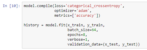
In this section, we'll set up learning and optimization functions, compile the model, fit it to training and testing data, and then actually run the model and see an animation indicating the effects on loss and accuracy.

In the following screenshot, we are compiling our model with loss, optimizer, and metrics:

Compiling model

The loss function is a mathematical function that tells optimizer how well it's doing. An optimizer function is a mathematical program that searches the available parameters in order to minimize the loss function. The metrics parameter are outputs from your machine learning model that should be human readable so that you can understand how well your model is running. Now, these loss and optimizer parameters are laden with math. By and large, you can approach this as a cookbook. When you are running a machine learning model with Keras, you...

Hyperparameters

In this section, we'll explore hyperparameters, or parameters that can't quite be machine learned.

We'll also cover trainable parameters (these are the parameters that are learned by the solver), nontrainable parameters (additional parameters in the models that don't require training), and then finally, hyperparameters (parameters that aren't learned by a traditional solver).

In our Model summary output screenshot, pay attention to the number of trainable parameters in the highlighted section of code at the bottom of the screenshot. That is the number of individual floating-point numbers that are contained inside of our model that our adam optimizer, in conjunction with our categorical cross-entropy loss function, will be exploring in order to find the best parameter values possible. So, this trainable parameter number is the only set of...

Grid searches

In this section, we will explore grid searches.

We'll talk a bit about optimization versus grid searching, setting up a model generator function, setting up a parameter grid and doing a grid search with cross-validation, and finally, reporting the outcomes of our grid search so we can pick the best model.

So why, fundamentally, are there two different kinds of machine learning activities here? Well, optimization solves for parameters with feedback from a loss function: it's highly optimized. Specifically, a solver doesn't have to try every parameter value in order to work. It uses a mathematical relationship with partial derivatives in order to move along what is called a gradient. This lets it go essentially downhill mathematically to find the right answer.

Grid searching isn't quite so smart. In fact, it's completely brute force. When we...

Summary

In this chapter, we actually covered an awful lot of material. We saw the structure of the classical or dense neural network. We learned about activation and nonlinearity, and we learned about softmax. We then set up testing and training data and we learned how to construct the network with Dropout and Flatten. We also learned all about solvers, or how machine learning actually learns. We then explored hyperparameters, and finally, we fine-tuned our model with grid search.

In the next chapter, we'll take what we've learned and alter the structure of our network to build what is called a convolutional neural network (CNN).