Chapter 3. Simulating a Model

In this chapter, we'll learn how to simulate a model. We'll start with a little theory about the solver and simulation time in order to understand the main concepts behind the Simulink engine. Then we will assemble the test system by putting together the cruise controller and the car model, and run various simulations. We'll be able to calibrate our cruise controller and we'll learn what really sets Simulink apart—many different source blocks and one mighty sink block, Scope.

The mandatory theory

Before starting the simulation, we'll have a closer look at how Simulink computes the simulation results, in order to be able to choose the appropriate simulation time and solver.

Let's build a simple system that finds the solution to this problem:

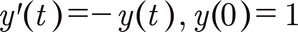
The exact mathematical solution is y(t) = e ^-t.

The Simulink model (which we'll save as example.slx) that implements the problem is:

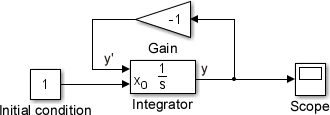
Notice that we've set the Initial condition source parameter of the Integrator block to be external.

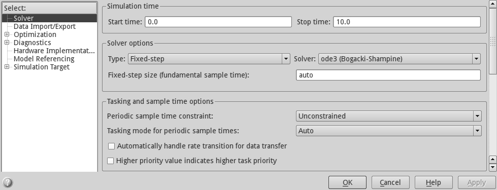
To configure the simulation time and solver of this model, click on the Model Configuration Parameters option from the Simulation menu (keyboard shortcut: Ctrl + E).

A new window will open; select the Solver node from the left-side panel, which will give you access to configure the Solver options and Simulation time parameters.

Under the Solver options section, select the Type list value as Fixed-step (don't worry, we'll explain the meaning later) as shown in the following screenshot:

Then let's edit...

Build the complete closed-loop system

So far we've got two models: a simple cruise controller and a beautiful car. Until now, they've been treated separately in an open loop. Remembering what we learned in the previous chapter, we're going to place the required blocks and connect them in a closed loop.

Let's open both the models and copy them to a new model named cruise_control_sim.slx. If their workspaces aren't loaded automatically, load them by dragging them from their folders to the MATLAB's Command Window and save the new workspace as cruise_control_sim.mat. It's suggested to have the new workspace loaded automatically via the PreLoadFcn model callback as we have learned in the previous chapter.

In order to see what's happening inside the engine, let's pull out the Gear and RPM signals from Alfa Romeo 147 GTA | Engine force | Gearbox and differential until we reach the root block, by adding and connecting the output ports to every parent subsystem.

Then we need to make the important connections...

Configuring the simulation

First and foremost, with the knowledge we gained in this chapter, we have to choose the right simulation times, the solvers, and their options. Let's open the model's Configuration Parameters window (or press Ctrl + E) for the last time.

Simulation times

The Start time parameter will be left as 0.0 seconds. We're not going to wait at the car parking, are we?

Having a powerful engine, we'll reach the target speed of 100 km/h from standstill in less than 10 seconds. But we want to see how the vehicle speed settles to the target speed (to detect overshoots and make sure the target is actually reached), so we'll use a long enough Stop time, 50 seconds.

The step size will be large enough to allow an external (soft real-time) application to run synchronously but small enough to not allow the car to reach a speed higher than the target before the cruise control can cut the throttle. This happens when the target speed is low and the car is in the first gear and jumps from...

Run our first serious simulation

Let's place a Step block in the model, connect it to the Target Goto (whose corresponding From block is connected to the Target speed controller input), and set its Final value to 100 km/h.

Run the simulation and open the Scope block. The speed graph should be like this one:

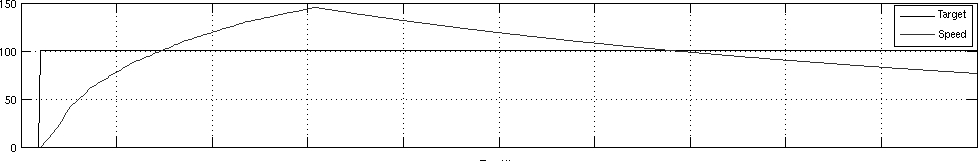
Quite an overshoot! The vehicle speed reaches almost 150 km/h when the controller closes the throttle. This is due to a too high integral gain, K_i, forcing the vehicle to go a lot faster than intended. Who wants a ride?

Calibrate the PI controller

To calibrate the PI controller constants, K_p and K_i, we'll use this manual method of keeping K_i to zero and finding the K_p value to where the Throttle signal begins to oscillate.

Then we'll halve the found value and save it into K_p and tune K_i in order to reach the target speed with a minimum overshoot.

Calibrating K_p

Prepare the model by setting K_i to zero with this MATLAB command: Ki = 0.

We'll start with an insanely high proportional gain value,...

Test with other sources

So far we've learned how to use the Step source block. This is arguably the most important source because it presents clearly the system's transient answer to a stimulus.

But that's about it; it doesn't show the response to a wave, a random signal, or a noise.

A more thorough test with other sources could help us detect problems that were overlooked. For instance, we didn't take into account while testing that the car can show a very different response in lower gears: at 100 km/h, it was running in fourth gear.

Sine Wave

The cruise controller is acting only on the throttle, so we can predict that it will be hard for it to follow decreasing speeds.

Let's try using a Sine Wave block as the target speed source, which was configured as follows:

• Bias: 100 (km/h)

• Amplitude: 20 (km/h)

• Frequency: 0.2 (rad/s)

The simulation result is shown as follows:

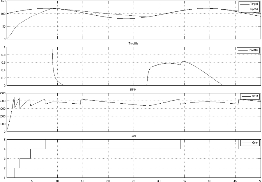
Our cruise controller can't use the brakes, so it isn't able to follow the falling side of the wave. But it's able to rise up fast...

Summary

You are now able to prepare a Simulink virtual test bench and run the closed-loop simulations of a controller and the mathematical model of the controlled item by setting the right simulation parameters, choosing the most appropriate sources, and viewing the result on the Scope block.

In the next chapter, you'll learn how to use your Simulink models with something outside Simulink itself. Have you got a spare car?