Reader small image

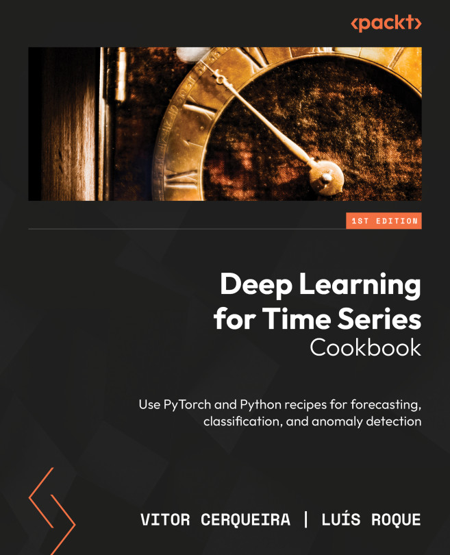
You're reading from  Deep Learning for Time Series Cookbook

Product typeBook
Published inMar 2024
PublisherPackt
ISBN-139781805129233
Edition1st Edition
Right arrow
Authors (2):
Vitor Cerqueira
Vitor Cerqueira
author image
Vitor Cerqueira

​Vitor Cerqueira is a time series researcher with an extensive background in machine learning. Vitor obtained his Ph.D. degree in Software Engineering from the University of Porto in 2019. He is currently a Post-Doctoral researcher in Dalhousie University, Halifax, developing machine learning methods for time series forecasting. Vitor has co-authored several scientific articles that have been published in multiple high-impact research venues.
Read more about Vitor Cerqueira

Luís Roque
Luís Roque
author image
Luís Roque

Luís Roque, is the Founder and Partner of ZAAI, a company focused on AI product development, consultancy, and investment in AI startups. He also serves as the Vice President of Data & AI at Marley Spoon, leading teams across data science, data analytics, data product, data engineering, machine learning operations, and platforms. In addition, he holds the position of AI Advisor at CableLabs, where he contributes to integrating the broadband industry with AI technologies. Luís is also a Ph.D. Researcher in AI at the University of Porto's AI&CS lab and oversees the Data Science Master's program at Nuclio Digital School in Barcelona. Previously, he co-founded HUUB, where he served as CEO until its acquisition by Maersk.
Read more about Luís Roque

View More author details
Right arrow

Univariate Time Series Forecasting

In this chapter, we’ll develop deep learning models to tackle univariate time series forecasting problems. We’ll touch on several aspects of time series preprocessing, such as preparing a time series for supervised learning and dealing with conditions such as trend or seasonality.

We’ll cover different types of models, including simple baselines such as the naïve or historical mean method. We’ll provide a brief background on a popular forecasting technique, autoregressive integrated moving average (ARIMA). Then, we’ll explain how to create a forecasting model using different types of deep learning methods. These include feedforward neural networks, long short-term memory (LSTM), gated recurrent units (GRU), Stacked LSTM, and convolutional neural networks (CNNs). You will also learn how to deal with common problems that arise in time series modeling; for example, how to deal with trend using first differences...
Technical requirements

Before diving into univariate time series forecasting problems, we need to ensure that we have the appropriate software and libraries installed on our system. Here, we’ll go over the main technical requirements for implementing the procedures described in this chapter:

  • We will primarily need Python 3.9 or a later version, pip or Anaconda, PyTorch, and CUDA (optional). You can check the Installing PyTorch recipe from the previous chapter for more information on these.
  • NumPy (1.26.3) and pandas (2.1.4): Both these Python libraries provide several methods for data manipulation and analysis.
  • statsmodels (0.14.1): This library implements several statistical methods, including a few useful time series analysis techniques.
  • scikit-learn (1.4.0): scikit-learn is a popular Python library for statistical learning. It contains several methods to solve different tasks, such as classification, regression, and clustering.
  • sktime (0.26.0): A Python...

Building simple forecasting models

Before diving into more complex methods, let’s get started with some simple forecasting models: the naive, seasonal naive, and mean models.

Getting ready

In this chapter, we focus on forecasting problems involving univariate time series. Let’s start by loading one of the datasets we explored in Chapter 1:

import pandas as pd
serie = pd.read_csv(
    "assets/datasets/time_series_solar.csv",
    parse_dates=["Datetime"],
    index_col="Datetime",
)['Incoming Solar']

In the preceding code, series is a pandas Series object that contains the univariate time series.

How to do it…

We can now forecast our time series using the three following methods:

  • Naive: The simplest forecasting method is the naive approach. This method assumes that the next observation is the same as the last one. In Python, it could be implemented as...

Univariate forecasting with ARIMA

ARIMA is a univariate time series forecasting method based on two components: an autoregression part and a moving average part. In autoregression, a lag refers to a previous point or points in the time series data that are used to predict future values. For instance, if we’re using a lag of one, we’d use the value observed in the previous time step to model a given observation. The moving average part uses past errors to model the future observations of the time series.

Getting ready

To work with the ARIMA model, you’ll need to install the statsmodels Python package if it’s not already installed. You can install it using pip:

pip install -U statsmodels

For this recipe, we’ll use the same dataset as in the previous recipe.

How to do it…

In Python, you can use the ARIMA model from the statsmodels library. Here’s a basic example of how to fit an ARIMA model:

import pandas as pd
from...

Preparing a time series for supervised learning

In this recipe, we turn our attention to machine learning approaches to forecasting. We start by describing the process of transforming a time series from a sequence of values into a format suitable for supervised learning.

Getting ready

Supervised learning involves a dataset with explanatory variables (input) and a target variable (output). A time series comprises a sequence of values with an associated timestamp. Therefore, we need to restructure the time series for supervised learning. A common approach to do this is using a sliding window. Each value of the series is based on the recent past values before it (also called lags).

To prepare for this section, you need to have your time series data available in a pandas DataFrame and have the pandas and NumPy libraries installed. If not, you can install them using pip:

pip install -U pandas numpy

We also load the univariate time series into the Python session:

series...

Univariate forecasting with a feedforward neural network

This recipe walks you through the process of building a feedforward neural network for forecasting with univariate time series.

Getting ready

Having transformed the time series data into an appropriate format for supervised learning, we are now ready to employ it for training a feedforward neural network. We strategically decided to resample the dataset, transitioning from hourly to daily data. This optimization significantly accelerates our training processes:

series = series.resample('D').sum()

How to do it…

Here are the steps for building and evaluting a feedforward neural network using PyTorch:

  1. We begin by splitting the data into training and testing and normalizing them. It’s important to note that the scaler should be fitted on the training set and used to transform both the training and test sets:
    import pandas as pd
    from sklearn.model_selection import train_test_split
    from...

Univariate forecasting with an LSTM

This recipe walks you through the process of building an LSTM neural network for forecasting with univariate time series.

Getting ready

As we saw in Chapter 2, LSTM networks, a variant of RNNs, have gained substantial attention for their performance on time series and sequence data. LSTM networks are particularly suited for this task because they can effectively capture long-term temporal dependencies in the input data due to their inherent memory cells.

This section will extend our univariate time series forecasting to LSTM networks using PyTorch. So, we continue with the objects created in the previous recipe (Univariate forecasting with a feedforward neural network).

How to do it…

We will use the same train and test sets from the previous section. For an LSTM, we must reshape the input data to 3D. As we explored in the previous chapter, the three dimensions of the input tensor to LSTMs represent the following aspects:

...

Univariate forecasting with a GRU

This recipe walks you through the process of building a GRU neural network for forecasting with univariate time series.

Getting ready

Now that we have seen how LSTMs can be used for univariate time series forecasting, let’s now shift our attention to another type of RNN architecture known as GRU. GRUs, like LSTMs, are designed to capture long-term dependencies in sequence data effectively but do so with a slightly different and less complex internal structure. This often makes them faster to train.

For this section, we will use the same training and testing sets as in the previous sections. Again, the input data should be reshaped into a 3D tensor with dimensions representing observations, time steps, and features respectively:

X_train = X_train.view([X_train.shape[0], X_train.shape[1], 1])
X_test = X_test.view([X_test.shape[0], X_test.shape[1], 1])

How to do it…

Let’s start constructing a GRU network with the...

Univariate forecasting with a Stacked LSTM

This recipe walks you through the process of building an LSTM neural network with multiple layers for forecasting with univariate time series.

Getting ready

For complex time series prediction problems, one LSTM layer may not be sufficient. In this case, we can use a stacked LSTM, which is essentially multiple layers of LSTM stacked one on top of the other. This can provide a higher level of input abstraction and may lead to improved prediction performance.

We will continue to use the same reshaped train and test sets from the previous recipe:

X_train = X_train.view([X_train.shape[0], X_train.shape[1], 1])
X_test = X_test.view([X_test.shape[0], X_test.shape[1], 1])

We also use the LSTM neural network defined in the Univariate forecasting with an LSTM recipe:

class LSTM(nn.Module):
    def __init__(self, input_dim, hidden_dim, num_layers, output_dim):
        super...

Combining an LSTM with multiple fully connected layers

Sometimes, it may be valuable to combine different types of neural networks in a single model. In this recipe, you’ll learn how to combine an LSTM module with a fully connected layer that is the basis of feedforward neural networks.

Getting ready

In this section, we’ll use a hybrid model that combines an LSTM layer with multiple fully connected (also known as dense) layers. This allows us to further abstract features from the sequence, and then learn complex mappings to the output space.

We continue using the reshaped train and test sets from the previous sections.

How to do it…

To construct this hybrid model in PyTorch, we add two fully connected layers after the LSTM layer:

class HybridLSTM(nn.Module):
    def __init__(self, input_dim, hidden_dim, 
        output_dim=1, num_layers=1):
       &...

Univariate forecasting with a CNN

Now, we turn our attention to convolutional neural networks that have also shown promising results with time series data. Let’s learn how these methods can be used for univariate time series forecasting.

Getting ready

CNNs are commonly used in problems involving images, but they can also be applied to time series forecasting tasks. By treating time series data as a “sequence image,” CNNs can extract local features and dependencies from the data. To implement this, we’ll need to prepare our time series data similarly to how we did for LSTM models.

How to do it…

Let’s define a simple CNN model in PyTorch. For this example, we will use a single convolutional layer followed by a fully connected layer:

class CNNTimeseries(nn.Module):
    def __init__(self, input_dim, output_dim=1):
        super(CNNTimeseries, self).__init__()
  ...

Handling trend – taking first differences

In Chapter 1, we learned about different time series patterns such as trend or seasonality. This recipe describes the process of dealing with trend in time series before training a deep neural network.

Getting ready

As we learned in Chapter 1, trend is the long-term change in the time series. When the average value of the time series changes, this means that the data is not stationary. Non-stationary time series are more difficult to model, so it’s important to transform the data into a stationary series.

Trend is usually removed from the time series by taking the first differences until the data becomes stationary.

First, let’s start by splitting the time series into training and testing sets:

from sklearn.model_selection import train_test_split
train, test = train_test_split(series, test_size=0.2, shuffle=False)

We leave the last 20% of observations for testing.

How to do it…

There are two...

Handling seasonality – seasonal dummies and Fourier series

In this recipe, we’ll describe how to deal with seasonality in time series using seasonal dummy variables and a Fourier series.

Getting ready

Seasonality represents repeatable patterns that recur over a given period, such as every year. Seasonality is an important piece of time series, and it is important to capture it. The consensus in the literature is that neural networks cannot capture seasonal effects optimally. The best way to model seasonality is by feature engineering or data transformation. One way to handle seasonality is to add extra information that captures the periodicity of patterns. This can be done with seasonal dummies or a Fourier series.

We start by preparing the data using the series_to_supervised() function:

train, test = train_test_split(series, test_size=0.2, shuffle=False)
scaler = MinMaxScaler(feature_range=(-1, 1))
train_norm = scaler.fit_transform(
    ...

Handling seasonality – seasonal differencing

In this recipe, we show how differencing can be used to model seasonal patterns in time series.

Getting ready

We’ve learned to use first differences to remove the trend from time series. Differencing can also work for seasonality. But, instead of taking the difference between consecutive observations, for each point, you subtract the value of the previous observation from the same season. For example, suppose you’re modeling monthly data. You perform seasonal differencing by subtracting the value of February of the previous year from the value of February of the current year.

The process is similar to what we did with first differences to remove the trend. Let’s start by loading the data:

time_series = df["Incoming Solar"]
train, test = train_test_split(time_series, test_size=0.2, shuffle=False)

In this recipe, we’ll use seasonal differencing to remove yearly seasonality.

How...

Handling seasonality – seasonal decomposition

This recipe describes yet another approach to modeling seasonality, this time using a time series decomposition approach.

Getting ready

We learned about time series decomposition methods in Chapter 1. Decomposition methods aim at extracting the individual parts that make up a time series.

We can use this approach to deal with seasonality. The idea is to separate the seasonal component from the rest (trend plus residuals). We can use a deep neural network to model the seasonally adjusted series. Then, we use a simple model to forecast the seasonal component.

Again, we’ll start with the daily solar radiation time series. This time, we won’t split training and testing to show how the forecasts are obtained in practice.

How to do it…

We start by decomposing the time series using STL. We learned about this method in Chapter 1:

from statsmodels.tsa.api import STL
series_decomp = STL(series, period...

Handling non-constant variance – log transformation

We’ve learned how to deal with changes in the level of the time series that occur due to either trend or seasonal patterns. In this recipe, we’ll deal with changes in the variance of time series.

Getting ready

We’ve learned in Chapter 1 that some time series are heteroscedastic, which means that the variance changes over time. Non-constant variance is problematic as it makes the learning process more difficult.

Let’s start by splitting the solar radiation time series into training and testing sets:

train, test = train_test_split(time_series, test_size=0.2, 
    shuffle=False)

Again, we leave the last 20% of observations for testing.

How to do it…

We’ll show how to stabilize the variance of a time series using the logarithm transformation and a Box-Cox power transformation.

Log transformation

In Chapter 1, we defined the LogTransformation...

lock icon
The rest of the chapter is locked
You have been reading a chapter from
Deep Learning for Time Series Cookbook
Published in: Mar 2024Publisher: PacktISBN-13: 9781805129233
Register for a free Packt account to unlock a world of extra content!
A free Packt account unlocks extra newsletters, articles, discounted offers, and much more. Start advancing your knowledge today.
undefined
Unlock this book and the full library FREE for 7 days
Get unlimited access to 7000+ expert-authored eBooks and videos courses covering every tech area you can think of
Renews at $15.99/month. Cancel anytime

Authors (2)

author image
Vitor Cerqueira

​Vitor Cerqueira is a time series researcher with an extensive background in machine learning. Vitor obtained his Ph.D. degree in Software Engineering from the University of Porto in 2019. He is currently a Post-Doctoral researcher in Dalhousie University, Halifax, developing machine learning methods for time series forecasting. Vitor has co-authored several scientific articles that have been published in multiple high-impact research venues.
Read more about Vitor Cerqueira

author image
Luís Roque

Luís Roque, is the Founder and Partner of ZAAI, a company focused on AI product development, consultancy, and investment in AI startups. He also serves as the Vice President of Data & AI at Marley Spoon, leading teams across data science, data analytics, data product, data engineering, machine learning operations, and platforms. In addition, he holds the position of AI Advisor at CableLabs, where he contributes to integrating the broadband industry with AI technologies. Luís is also a Ph.D. Researcher in AI at the University of Porto's AI&CS lab and oversees the Data Science Master's program at Nuclio Digital School in Barcelona. Previously, he co-founded HUUB, where he served as CEO until its acquisition by Maersk.
Read more about Luís Roque