Search icon
Arrow left icon
All Products
Best Sellers
New Releases
Books
Videos
Audiobooks
Learning Hub
Newsletters
Free Learning
Arrow right icon
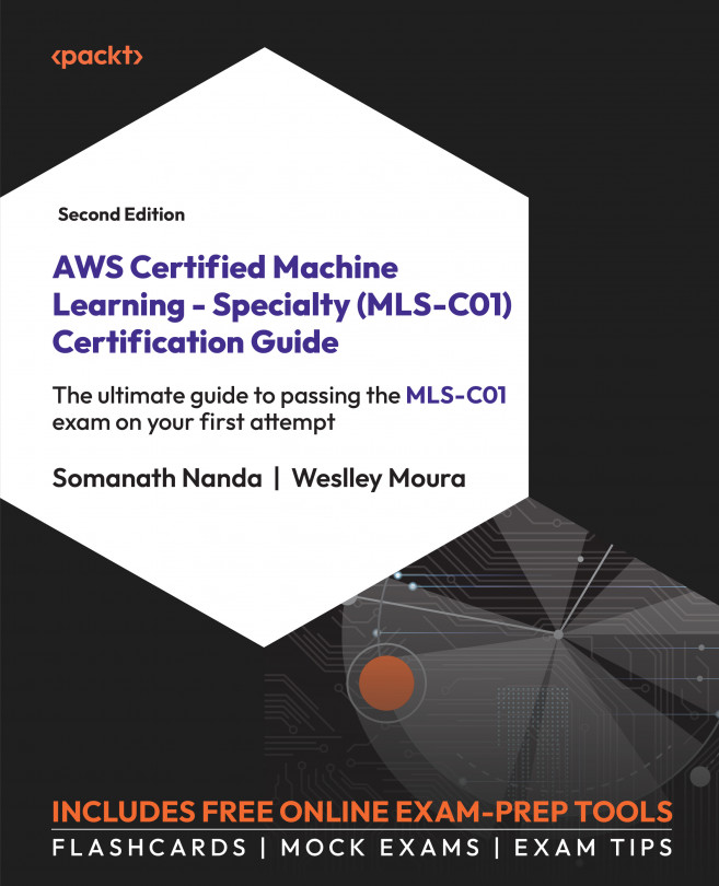
AWS Certified Machine Learning - Specialty (MLS-C01) Certification Guide - Second Edition

AWS Certified Machine Learning - Specialty (MLS-C01) Certification Guide: The ultimate guide to passing the MLS-C01 exam on your first attempt, Second Edition

By Somanath Nanda , Weslley Moura
₱1,836.99 ₱1,284.99
Book Feb 2024 342 pages 2nd Edition
eBook
₱1,836.99 ₱1,284.99
Print
₱2,296.99
Subscription
Free Trial
eBook
₱1,836.99 ₱1,284.99
Print
₱2,296.99
Subscription
Free Trial

What do you get with eBook?

Product feature icon Instant access to your Digital eBook purchase
Product feature icon Download this book in EPUB and PDF formats
Product feature icon Access this title in our online reader with advanced features
Product feature icon DRM FREE - Read whenever, wherever and however you want
Buy Now

Product Details


Publication date : Feb 29, 2024
Length 342 pages
Edition : 2nd Edition
Language : English
ISBN-13 : 9781835082201
Category :
Table of content icon View table of contents Preview book icon Preview Book

AWS Certified Machine Learning - Specialty (MLS-C01) Certification Guide - Second Edition

Machine Learning Fundamentals

For many decades, researchers have been trying to simulate human brain activity through the field known as artificial intelligence, or AI for short. In 1956, a group of people met at the Dartmouth Summer Research Project on Artificial Intelligence, an event that is widely accepted as the first group discussion about AI as it’s known today. Researchers were trying to prove that many aspects of the learning process could be precisely described and, therefore, automated and replicated by a machine. Today, you know they were right!

Many other terms appeared in this field, such as machine learning (ML) and deep learning (DL). These sub-areas of AI have also been evolving for many decades (granted, nothing here is new to the science). However, with the natural advance of the information society and, more recently, the advent of big data platforms, AI applications have been reborn with much more applicability – power (because now there are more computational resources to simulate and implement them) and applicability (because now information is everywhere).

Even more recently, cloud service providers have put AI in the cloud. This helps all sizes of companies to reduce their operational costs and even lets them sample AI applications, considering that it could be too costly for a small company to maintain its own data center to scale an AI application.

An incredible journey of building cutting-edge AI applications has emerged with the popularization of big data and cloud services. In June 2020, one specific technology gained significant attention and put AI on the list of the most discussed topics across the technology industry – its name is ChatGPT.

ChatGPT is a popular AI application that uses large language models (more specifically, generative pre-trained transformers) trained on massive amounts of text data to understand and generate human-like language. These models are designed to process and comprehend the complexities of human language, including grammar, context, and semantics.

Large language models utilize DL techniques (for example, deep neural networks based on transformer architecture) to learn patterns and relationships within textual data. They consist of millions of parameters, making them highly complex and capable of capturing very specific language structures.

Such mixing of terms and different classes of use cases might get one stuck on understanding the practical steps of implementing AI applications. That brings you to the goal of this chapter: being able to describe what the terms AI, ML, and DL mean, as well as understanding all the nuances of an ML pipeline. Avoiding confusion about these terms and knowing what exactly an ML pipeline is will allow you to properly select your services, develop your applications, and master the AWS Machine Learning Specialty exam.

Making the Most Out of this Book – Your Certification and Beyond

This book and its accompanying online resources are designed to be a complete preparation tool for your MLS-C01 Exam.

The book is written in a way that you can apply everything you’ve learned here even after your certification. The online practice resources that come with this book (Figure 1.1) are designed to improve your test-taking skills. They are loaded with timed mock exams, interactive flashcards, and exam tips to help you work on your exam readiness from now till your test day.

Before You Proceed

To learn how to access these resources, head over to Chapter 11, Accessing the Online Practice Resources, at the end of the book.

Figure 1.1 – Dashboard interface of the online practice resources

Figure 1.1 – Dashboard interface of the online practice resources

Here are some tips on how to make the most out of this book so that you can clear your certification and retain your knowledge beyond your exam:

  1. Read each section thoroughly.
  2. Make ample notes: You can use your favorite online note-taking tool or use a physical notebook. The free online resources also give you access to an online version of this book. Click the BACK TO THE BOOK link from the Dashboard to access the book in Packt Reader. You can highlight specific sections of the book there.
  3. Chapter Review Questions: At the end of this chapter, you’ll find a link to review questions for this chapter. These are designed to test your knowledge of the chapter. Aim to score at least 75% before moving on to the next chapter. You’ll find detailed instructions on how to make the most of these questions at the end of this chapter in the Exam Readiness Drill - Chapter Review Questions section. That way, you’re improving your exam-taking skills after each chapter, rather than at the end.
  4. Flashcards: After you’ve gone through the book and scored 75% more in each of the chapter review questions, start reviewing the online flashcards. They will help you memorize key concepts.
  5. Mock Exams: Solve the mock exams that come with the book till your exam day. If you get some answers wrong, go back to the book and revisit the concepts you’re weak in.
  6. Exam Tips: Review these from time to time to improve your exam readiness even further.

The main topics of this chapter are as follows:

  • Comparing AI, ML, and DL
  • Classifying supervised, unsupervised, and reinforcement learning
  • The CRISP-DM modeling life cycle
  • Data splitting
  • Modeling expectations
  • Introducing ML frameworks
  • ML in the cloud

Comparing AI, ML, and DL

AI is a broad field that studies different ways to create systems and machines that will solve problems by simulating human intelligence. There are different levels of sophistication to create these programs and machines, which go from simple rule-based engines to complex self-learning systems. AI covers, but is not limited to, the following sub-areas:

  • Robotics
  • Natural language processing (NLP)
  • Rule-based systems
  • Machine learning (ML)
  • Computer vision

The area this certification exam focuses on is ML.

Examining ML

ML is a sub-area of AI that aims to create systems and machines that can learn from experience, without being explicitly programmed. As the name suggests, the system can observe its underlying environment, learn, and adapt itself without human intervention. Algorithms behind ML systems usually extract and improve knowledge from the data and conditions that are available to them.

Figure 1.2 – Hierarchy of AI, ML, and DL

Figure 1.2 – Hierarchy of AI, ML, and DL

You should keep in mind that there are different classes of ML algorithms. For example, decision tree-based models, probabilistic-based models, and neural network models. Each of these classes might contain dozens of specific algorithms or architectures (some of them will be covered in later sections of this book).

As you might have noticed in Figure 1.2, you can be even more specific and break the ML field down into another very important topic for the Machine Learning Specialty exam: deep learning, or DL for short.

Examining DL

DL is a subset of ML that aims to propose algorithms that connect multiple layers to solve a particular problem. The knowledge is then passed through, layer by layer, until the optimal solution is found. The most common type of DL algorithm is deep neural networks.

At the time of writing this book, DL is a very hot topic in the field of ML. Most of the current state-of-the-art algorithms for machine translation, image captioning, and computer vision were proposed in the past few years and are a part of the DL field (GPT-4, used by the ChatGPT application, is one of these algorithms).

Now that you have an overview of types of AI, take a look at some of the ways you can classify ML.

Classifying supervised, unsupervised, and reinforcement learning

ML is a very extensive field of study; that’s why it is very important to have a clear definition of its sub-divisions. From a very broad perspective, you can split ML algorithms into two main classes: supervised learning and unsupervised learning.

Introducing supervised learning

Supervised algorithms use a class or label (from the input data) as support to find and validate the optimal solution. In Table 1.1, there is a dataset that aims to classify fraudulent transactions from a financial company.

Day of the week

Hour

Transaction amount

Merchant type

Is fraud?

Mon

09:00

$1000

Retail

No

Tue

23:00

$5500

E-commerce

Yes

Fri

14:00

$500

Travel

No

Mon

10:00

$100

Retail

No

Tue

22:00

$100

E-commerce

No

Tue

22:00

$6000

E-commerce

Yes

Table 1.1 – Sample dataset for supervised learning

The first four columns are known as features or independent variables, and they can be used by a supervised algorithm to find fraudulent patterns. For example, by combining those four features (day of the week, EST hour, transaction amount, and merchant type) and six observations (each row is technically one observation), you can infer that e-commerce transactions with a value greater than $5,000 and processed at night are potentially fraudulent cases.

Important note

In a real scenario, you will have more observations in order to have statistical support to make this type of inference.

The key point is that you were able to infer a potential fraudulent pattern just because you knew, a priori, what is fraud and what is not fraud. This information is present in the last column of Table 1.1 and is commonly referred to as a target variable, label, response variable, or dependent variable. If the input dataset has a target variable, you should be able to apply supervised learning.

In supervised learning, the target variable might store different types of data. For instance, it could be a binary column (yes or no), a multi-class column (class A, B, or C), or even a numerical column (any real number, such as a transaction amount). According to the data type of the target variable, you will find which type of supervised learning your problem refers to. Table 1.2 shows how to classify supervised learning into two main groups: classification and regression algorithms:

Data type of the target variable

Sub data type of the target variable

Type of supervised learning applicable

Categorical

Binary

Binary classification

Categorical

Multi class

Multi classification

Numerical

N/A

Regression

Table 1.2 – Choosing the right type of supervised learning given the target variable

While classification algorithms predict a class (either binary or multiple classes), regression algorithms predict a real number (either continuous or discrete).

Understanding data types is important to make the right decisions on ML projects. You can split data types into two main categories: numerical and categorical data. Numerical data can then be split into continuous or discrete subclasses, while categorical data might refer to ordinal or nominal data:

  • Numerical/discrete data refers to individual and countable items (for example, the number of students in a classroom or the number of items in an online shopping cart).
  • Numerical/continuous data refers to an infinite number of possible measurements and they often carry decimal points (for example, temperature).
  • Categorical/nominal data refers to labeled variables with no quantitative value (for example, name or gender).
  • Categorical/ordinal data adds a sense of order to a labeled variable (for example, education level or employee title level).

In other words, when choosing an algorithm for your project, you should ask yourself: do I have a target variable? Does it store categorical or numerical data? Answering these questions will put you in a better position to choose a potential algorithm that will solve your problem.

However, what if you don’t have a target variable? In that case, you are facing an unsupervised learning problem. Unsupervised problems do not provide labeled data; instead, they provide all the independent variables (or features) that will allow unsupervised algorithms to find patterns in the data. The most common type of unsupervised learning is clustering, which aims to group the observations of the dataset into different clusters, purely based on their features. Observations from the same cluster are expected to be similar to each other, but very different from observations from other clusters. Clustering will be covered in more detail in future chapters of this book.

Semi-supervised learning is also present in the ML literature. This type of algorithm can learn from partially labeled data (some observations contain a label and others do not).

Finally, another learning approach that has been taken by another class of ML algorithms is reinforcement learning. This approach rewards the system based on the good decisions that it has made autonomously; in other words, the system learns by experience.

You have been learning about approaches and classes of algorithms at a very broad level. However, it is time to get specific and introduce the term model.

The CRISP-DM modeling life cycle

Modeling is a very common term used in ML when you want to specify the steps taken to solve a particular problem. For example, you could create a binary classification model to predict whether the transactions from Table 1.1 are fraudulent or not.

A model, in this context, represents all the steps to create a solution as a whole, which includes (but is not limited to) the algorithm. The Cross-Industry Standard Process for Data Mining, more commonly referred to as CRISP-DM, is one of the methodologies that provides guidance on the common steps that you should follow to create models. This methodology is widely used by the market and is covered in the AWS Machine Learning Specialty exam:

Figure 1.3 – CRISP-DM methodology

Figure 1.3 – CRISP-DM methodology

Everything starts with business understanding, which will produce the business objectives (including success criteria), situation assessment, data mining goals, and project plan (with an initial assessment of tools and techniques). During the situation assessment, you should also look into an inventory of resources, requirements, assumptions and constraints, risks, terminology, costs, and benefits. Every single assumption and success criterion matters when you are modeling.

The next step is known as data understanding, where you will collect raw data, describe it, explore it, and check its quality. This is an initial assessment of the data that will be used to create the model. Again, data scientists must be skeptical. You must be sure you understand all the nuances of the data and its source.

The data preparation phase is actually the one that usually consumes most of the time during modeling. In this phase, you need to select and filter the data, clean it according to the task that needs to be performed, come up with new attributes, integrate the data with other data sources, and format it as expected by the algorithm that will be applied. These tasks are often called feature engineering.

Once the data is prepared, you can finally start the modeling phase. Here is where the algorithms come in. You should start by ensuring the selection of the right technique. Remember: according to the presence or absence of a target variable (and its data type), you will have different algorithms to choose from. Each modeling technique might carry some implicit assumptions of which you have to be aware. For example, if you choose a multiple linear regression algorithm to predict house prices, you should be aware that this type of model expects a linear relationship between the variables of your data.

There are hundreds of algorithms out there and each of them might have its own assumptions. After choosing the ones that you want to test in your project, you should spend some time checking their specifics. In later chapters of this book, you will learn about some of them.

Important note

Some algorithms incorporate in their logic a sub-process known as feature selection. This is a step where the most important features will be selected to build your best model. Decision trees are examples of algorithms that perform feature selection automatically. You will learn about feature selection in more detail later on, since there are different ways to select the best variables for your model.

During the modeling phase, you should also design a testing approach for the model, defining which evaluation metrics will be used and how the data will be split. With that in place, you can finally build the model by setting the hyperparameters of the algorithm and feeding the model with data. This process of feeding the algorithm with data to find a good estimator is known as the training process. The data used to feed the model is known as training data. There are different ways to organize the training and testing data, which you will learn about in this chapter.

Important note

ML algorithms are built of parameters and hyperparameters. Parameters are learned from the data; for example: a decision-tree-based algorithm might learn from the training data that a particular feature should compose its root level based on information gain assessments. Hyperparameters, on the other hand, are used to control the learning process. Taking the same example about decision trees, you could specify the maximum allowed depth of the tree (regardless of the training data). Hyperparameter tuning is a very important topic in the exam and will be covered in fine-grained detail later on.

Once the model is trained, you can evaluate and review the results in order to propose the next steps. If the results are not acceptable (based on business success criteria), you should go back to earlier steps to check what else can be done to improve the model’s results. It could either be the subtle tuning of the hyperparameters of the algorithm, a new data preparation step, or even the redefinition of business drivers. On the other hand, if the model quality is acceptable, you can move on to the deployment phase.

In this last phase of the CRISP-DM methodology, you have to think about the deployment plan, monitoring, and maintenance of the model. You can look at this step from two perspectives: training and inference. The training pipeline consists of those steps needed to train the model, which include data preparation, hyperparameter definition, data splitting, and model training itself. Somehow, you must store all the model artifacts somewhere, since they will be used by the next pipeline that needs to be developed: the inference pipeline.

The inference pipeline just uses model artifacts to execute the model against brand-new observations (data that has never been seen by the model during the training phase). For example, if the model was trained to identify fraudulent transactions, this is the time when new transactions will pass through the model to be classified.

In general, models are trained once (through the training pipeline) and executed many times (through the inference pipeline). However, after some time, it is expected that there will be some model degradation, also known as model drift. This phenomenon happens because the model is usually trained in a static training set that aims to represent the business scenario at a given point in time; however, businesses evolve, and it might be necessary to retrain the model on more recent data to capture new business aspects. That’s why it is important to keep tracking model performance even after model deployment.

The CRISP-DM methodology is so important to the context of the AWS Machine Learning Specialty exam that, if you look at the four domains covered by AWS, you will realize that they were generalized from the CRISP-DM stages: data engineering, exploratory data analysis, modeling, and ML implementation and operations.

You now understand all the key stages of a modeling pipeline and you know that the algorithm itself is just part of a larger process! Next, you will see how to split your data to create and validate ML models.

Data splitting

Training and evaluating ML models are key tasks of the modeling pipeline. ML algorithms need data to find relationships among features in order to make inferences, but those inferences need to be validated before they are moved to production environments.

The dataset used to train ML models is commonly called the training set. This training data must be able to represent the real environment where the model will be used; it will be useless if that requirement is not met.

Coming back to the fraud example presented in Table 1.1, based on the training data, you found that e-commerce transactions with a value greater than $5,000 and processed at night are potentially fraudulent cases. With that in mind, after applying the model in a production environment, the model is supposed to flag similar cases, as learned during the training process.

Therefore, if those cases only exist in the training set, the model will flag false positive cases in production environments. The opposite scenario is also true: if there is a particular fraud case in production data, not reflected in the training data, the model will flag a lot of false negative cases. False positive and false negative ratios are just two of many quality metrics that you can use for model validation. These metrics will be covered in much more detail later on.

By this point, you should have a clear understanding of the importance of having a good training set. Now, supposing you do have a valid training set, how could you have some level of confidence that this model will perform well in production environments? The answer is by using testing and validation sets:

Figure 1.4 – Data splitting

Figure 1.4 – Data splitting

Figure 1.4 shows the different types of data splitting that you can have during training and inference pipelines. The training data is used to create the model; the testing data is used to extract the final model quality metrics. The testing data cannot be used during the training process for any reason other than to extract model metrics.

The reason to avoid using the testing data during training is simple: you cannot let the model learn on top of the data that will be used to validate it. This technique of holding one piece of the data for testing is often called hold-out validation.

The box on the right side of Figure 1.4 represents the production data. Production data usually comes in continuously and you have to execute the inference pipeline in order to extract model results from it. No training, nor any other type of recalculation, is performed on top of production data; you just have to pass it through the inference pipeline as it is.

From a technical perspective, most ML libraries implement training steps with the .fit method, while inference steps are implemented by the .transform or .predict method. Again, this is just a common pattern used by most ML libraries, but be aware that you might find different name conventions across ML libraries.

Still looking at Figure 1.4, there is another box, close to the training data, named Validation data. This is a subset of the training set often used to support the creation of the best model, before moving on to the testing phase. You will learn about validation sets in much more detail, but first, you should understand why you need them.

Overfitting and underfitting

ML models might suffer from two types of fitting issues: overfitting and underfitting. Overfitting means that your model performs very well on the training data but cannot be generalized to other datasets, such as testing and, even worse, production data. In other words, if you have an overfitted model, it only works on your training data.

When you are building ML models, you want to create solutions that are able to generalize what they have learned and infer decisions on other datasets that follow the same data distribution. A model that only works on the data that it was trained on is useless. Overfitting usually happens due to the large number of features or the lack of configuration of the hyperparameters of the algorithm.

On the other hand, underfitted models cannot fit the data during the training phase. As a result, they are so generic that they can’t perform well within the training, testing, or production data. Underfitting usually happens due to the lack of good features/observations or due to the lack of time to train the model (some algorithms need more iterations to properly fit the model).

Both overfitting and underfitting need to be avoided. There are many modeling techniques to work around them. For instance, you will learn about the commonly used cross-validation technique and its relationship with the validation data box shown in Figure 1.4.

Applying cross-validation and measuring overfitting

Cross-validation is a technique where you split the training set into training and validation sets. The model is then trained on the training set and tested on the validation set. The most common cross-validation strategy is known as k-fold cross-validation, where k is the number of splits of the training set.

Using k-fold cross-validation and assuming the value of k equals 10, you are splitting the training set into 10 folds. The model will be trained and tested 10 times. On each iteration, it uses 9 splits for training and leaves one split for testing. After 10 executions, the evaluation metrics extracted from each iteration are averaged and will represent the final model performance during the training phase, as shown in Figure 1.5:

Figure 1.5 – Cross-validation in action

Figure 1.5 – Cross-validation in action

Another common cross-validation technique is known as leave-one-out cross-validation (LOOCV). In this approach, the model is executed many times and, within each iteration, one observation is separated for testing and all the others are used for training.

There are many advantages of using cross-validation during training:

  • You mitigate overfitting in the training data since the model is always trained on a particular chunk of data and tested on another chunk that hasn’t been used for training.
  • You avoid overfitting in the test data since there is no need to keep using the testing data to optimize the model.
  • You expose the presence of overfitting or underfitting. If the model performance in the training/validation data is very different from the performance observed in the testing data, something is wrong.

It might be worth diving into the third item on that list since it is widely covered in the AWS Machine Learning Specialty exam. For instance, assume you are creating a binary classification model, using cross-validation during training, and using a testing set to extract final metrics (hold-out validation). If you get 80% accuracy in the cross-validation results and 50% accuracy in the testing set, it means that the model was overfitted to the training set, and so cannot be generalized to the testing set.

On the other hand, if you get 50% accuracy in the training set and 80% accuracy in the testing set, there is a systemic issue in the data. It is very likely that the training and testing sets do not follow the same distribution.

Important note

Accuracy is a model evaluation metric commonly used on classification models. It measures how often the model made a correct decision during its inference process. That metric was selected just for the sake of demonstration, but be aware that there are many other evaluation metrics applicable for each type of model (which will be covered at the appropriate time).

Bootstrapping methods

Cross-validation is a good strategy to validate ML models, and you should try it in your daily activities as a data scientist. However, you should also know about other resampling techniques available out there. Bootstrapping is one of them.

While cross-validation works with no replacement, a bootstrapping approach works with replacement. With replacement means that, while you are drawing multiple random samples from a population dataset, the same observation might be duplicated across samples.

Usually, bootstrapping is not used to validate models as you do in the traditional cross-validation approach. The reason is simple: since it works with replacement, the same observation used for training could potentially be used for testing, too. This would result in inflated model performance metrics since the estimator is likely to be correct when predicting an observation that was already seen in the training set.

Bootstrapping is often used by ML algorithms in an embedded way that requires resampling capabilities to process the data. In this context, bootstrapping is not used to validate the model but to create the model. Random forest, which will be covered in Chapter 6, Applying Machine Learning Algorithms, is one of those algorithms that use bootstrapping internally for model building.

Designing a good data splitting/sampling strategy is crucial to the success of the model or the algorithm. You should come up with different approaches to split your data, check how the model is performing on each split, and make sure those splits represent the real scenario where the model will be used.

The variance versus bias trade-off

Any ML model is supposed to contain errors. There are three types of errors that you can find in models: bias errors, variance errors, and unexplained errors. The last one, as expected, cannot be explained. It is often related to the context of the problem and the relationships between the variables (you can’t control it).

The other two types of errors can be controlled during modeling. You can say that there is a trade-off between bias and variance errors because one will influence the other. In this case, increasing bias will decrease variance and vice versa.

Bias errors relate to assumptions taken by the model to learn the target function, the one that you want to solve. Some types of algorithms, such as linear algorithms, usually carry over that type of error because they make a lot of assumptions during model training. For example, linear models assume that the relationship present in the data is linear. Linear regression and logistic regression are types of algorithms that, in general, contain high bias. Decision trees, on the other hand, are types of algorithms that make fewer assumptions about the data and contain less bias.

Variance relates to the difference in estimations that the model performs on different training data. Models with high variance usually overfit the training set. Decision trees are examples of algorithms with high variance (they usually rely a lot on specifics of the training set, failing to generalize), and linear and logistic regression are examples of algorithms with low variance. It does not mean that decision trees are bad estimators; it just means that you need to prune (optimize) them during training.

That being said, the goal of any model is to minimize both bias and variance. However, as already mentioned, each one will impact the other in the opposite direction. For the sake of demonstration, consider a decision tree to understand how this trade-off works.

Decision trees are nonlinear algorithms and often contain low bias and high variance. In order to decrease variance, you can prune the tree and set the max_depth hyperparameter (the maximum allowed depth of the tree) to 10. That will force a more generic model, reducing variance. However, that change will also force the model to make more assumptions (since it is now more generic) and increase bias.

Shuffling your training set

Now that you know what variance and data splitting are, you can go a little deeper into the training dataset requirements. You are very likely to find questions around data shuffling in the exam. This process consists of randomizing your training dataset before you start using it to fit an algorithm.

Data shuffling will help the algorithm to reduce variance by creating a more generalizable model. For example, let’s say your training represents a binary classification problem and it is sorted by the target variable (all cases belonging to class “0” appear first, then all the cases belonging to class “1”).

When you fit an algorithm on this sorted data (especially some algorithms that rely on batch processing), it will make strong assumptions about the pattern of one of the classes, since it is very likely that it won’t be able to create random batches of data with a good representation of both classes. Once the algorithm builds strong assumptions about the training data, it might be difficult for it to change them.

Important note

Some algorithms are able to execute the training process by fitting the data in chunks, also known as batches. This approach lets the model learn more frequently since it will make partial assumptions after processing each batch of data (instead of making decisions only after processing the entire dataset).

On the other hand, there is no need to shuffle the testing set, since it will be used only by the inference process to check model performance.

Modeling expectations

So far, you have learned about model building, validation, and management. You can now complete the foundations of ML by learning about a couple of other expectations while modeling.

The first one is parsimony. Parsimony describes models that offer the simplest explanation and fit the best results when compared with other models. Here’s an example: while creating a linear regression model, you realize that adding 10 more features will improve your model’s performance by 0.001%. In this scenario, you should consider whether this performance improvement is worth the cost of parsimony (since your model will become more complex). Sometimes it is worth it, but most of the time it is not. You need to be skeptical and think according to your business case.

Parsimony directly supports interpretability. The simpler your model is, the easier it is to explain it. However, there is a battle between interpretability and predictivity: if you focus on predictive power, you are likely to lose some interpretability. Again, you must select what is the best situation for your use case.

Introducing ML frameworks

Being aware of some ML frameworks will put you in a much better position to pass the AWS Machine Learning Specialty exam. There is no need to master these frameworks since this is not a framework-specific certification; however, knowing some common terms and solutions will help you to understand the context of the problems/questions.

scikit-learn is probably the most popular ML framework that you should be aware of. It is an open source Python package that provides implementations of ML algorithms such as decision trees, support vector machines, linear regression, and many others. It also implements classes for data preprocessing, for example, one-hot encoding, label encoders, principal component analysis, and so on. All these preprocessing methods (and many others) will be covered in later sections of this book.

The downside of scikit-learn is the fact that it needs customization to scale up through multiple machines. There is another ML library that is very popular because of the fact that it can handle multiprocessing straight away: Spark’s ML library.

As the name suggests, it is an ML library that runs on top of Apache Spark, which is a unified analytical multi-processing framework used to process data on multiple machines. AWS offers a specific service that allows developers to create Spark clusters with a few clicks, known as EMR. Additionally, SageMaker (a fully managed ML service provided by AWS, which you will cover in a separate chapter) is well integrated with Apache Spark.

The Spark ML library is in constant development. As of the time of writing, it offers support to many ML classes of algorithms, such as classification and regression, clustering, and collaborative filtering. It also offers support for basic statistics computation, such as correlations and some hypothesis tests, as well as many data transformations, such as one-hot encoding, principal component analysis, min-max scaling, and others.

Another very popular ML framework is known as TensorFlow. This ML framework was created by the Google team and it is used for numerical computation and large-scale ML model development. TensorFlow implements not only traditional ML algorithms but also DL models.

TensorFlow is considered a low-level API for model development, which means that it can be very complex to develop more sophisticated models, such as transformers (for text mining). As an attempt to facilitate model development, other ML frameworks were built on top of TensorFlow to make it easier. One of these high-level frameworks is Keras. With Keras, developers can create complex DL models with just a few lines of code. More recently, Keras was incorporated into TensorFlow and it can be now called inside the TensorFlow library.

MXNet is another open source DL library. Using MXNet, you can scale up neural network-based models using multiple GPUs running on multiple machines. It also supports different programming languages, such as Python, R, Scala, and Java.

Graphical processing unit (GPU) support is particularly important in DL libraries such as TensorFlow and MXNet. These libraries allow developers to create and deploy neural network-based models with multiple layers. The training process of neural networks relies a lot on matrix operations, which perform much better on GPUs rather than on CPUs. That’s why these DL libraries commonly offer GPU support. AWS also offers EC2 instances with GPU enabled.

These ML frameworks need a special channel to communicate with GPU units. NVIDIA, the most common supplier of GPUs nowadays, has created an API called the Compute Unified Device Architecture (CUDA). CUDA is used to configure GPU units on NVIDIA devices; for example, setting up caching memory and the number of threads needed to train a neural network model. There is no need to master CUDA or GPU architecture for the AWS Machine Learning Specialty exam, but you definitely need to know what they are and how DL models take advantage of them.

Last, but not least, you should also be aware of some development frameworks widely used by the data science community, but not necessarily to create ML models. These frameworks interoperate with ML libraries to facilitate data manipulation and calculations. For example: pandas is a Python library that provides data processing capabilities and NumPy is an open source Python library that provides numerical computing.

These terms and libraries are so incorporated into data scientists’ daily routines that they might come up during the exam to explain some problem domain for you. Being aware of what they are will help you to quickly understand the context of the question.

ML in the cloud

ML has gone to the cloud and developers can now use it as a service. AWS has implemented ML services at different levels of abstraction. ML application services, for example, aim to offer out-of-the-box solutions for specific problem domains. AWS Lex is a very clear example of an ML application as a service, where people can implement chatbots with minimum development.

AWS Rekognition is another example, which aims to identify objects, people, text, scenes, and activities in images and videos. AWS provides many other ML application services, which will be covered in the next chapter of this book.

Apart from application services, AWS also provides ML development platforms, such as SageMaker. Unlike out-of-the-box services such as AWS Lex and Rekognition, SageMaker is a development platform that will let you build, train, and deploy your own models with much more flexibility.

SageMaker speeds up the development and deployment process by automatically handling the necessary infrastructure for the training and inference pipelines of your models. Behind the scenes, SageMaker orchestrates other AWS services (such as EC2 instances, load balancers, auto-scaling, and so on) to create a scalable environment for ML projects. SageMaker is probably the most important service that you should master for the AWS Machine Learning Specialty exam, and it will be covered in detail in a separate section. For now, you should focus on understanding the different approaches that AWS uses to offer ML-related services.

The third option that AWS offers for deploying ML models is the most generic and flexible one: you can deploy ML models by combining different AWS services and managing them individually. This essentially does what SageMaker does for you, building your applications from scratch. For example, you could use EC2 instances, load balancers, auto-scaling, and an API gateway to create an inference pipeline for a particular model. If you prefer, you can also use AWS serverless architecture to deploy your solution, for example, using AWS Lambda functions.

Summary

You are now heading toward the end of this chapter, in which you have learned about several important topics regarding the foundations of ML. You started the chapter with a theoretical discussion about AI, ML, and DL, and how this entire field has grown over the past few years due to the advent of big data platforms, cloud providers, and AI applications.

You then moved on to the differences between supervised, unsupervised, and reinforcement learning, highlighting some use cases related to each of them. This is likely to be a topic in the AWS Machine Learning Specialty exam.

You learned that an ML model is built in many different stages and the algorithm itself is just one part of the modeling process. You also learned about the expected behaviors of a good model.

You did a deep dive into data splitting, where you learned about different approaches to train and validate models, and you became aware of the mythic battle between variance and bias. You completed the chapter by getting a sense of ML frameworks and services.

Coming up next, you will learn about AWS application services for ML, such as Amazon Polly, Amazon Rekognition, Amazon Transcribe, and many other AI-related AWS services. But first, look at some sample questions to give you an idea of what you can expect in the exam.

Exam Readiness Drill – Chapter Review Questions

Apart from a solid understanding of key concepts, being able to think quickly under time pressure is a skill that will help you ace your certification exam. That is why working on these skills early on in your learning journey is key.

Chapter review questions are designed to improve your test-taking skills progressively with each chapter you learn and review your understanding of key concepts in the chapter at the same time. You’ll find these at the end of each chapter.

How To Access These Resources

To learn how to access these resources, head over to the chapter titled Chapter 11, Accessing the Online Practice Resources.

To open the Chapter Review Questions for this chapter, perform the following steps:

  1. Click the link – https://packt.link/MLSC01E2_CH01.

    Alternatively, you can scan the following QR code (Figure 1.6):

Figure 1.6 – QR code that opens Chapter Review Questions for logged-in users

Figure 1.6 – QR code that opens Chapter Review Questions for logged-in users

  1. Once you log in, you’ll see a page similar to the one shown in Figure 1.7:
Figure 1.7 – Chapter Review Questions for Chapter 1

Figure 1.7 – Chapter Review Questions for Chapter 1

  1. Once ready, start the following practice drills, re-attempting the quiz multiple times.

Exam Readiness Drill

For the first three attempts, don’t worry about the time limit.

ATTEMPT 1

The first time, aim for at least 40%. Look at the answers you got wrong and read the relevant sections in the chapter again to fix your learning gaps.

ATTEMPT 2

The second time, aim for at least 60%. Look at the answers you got wrong and read the relevant sections in the chapter again to fix any remaining learning gaps.

ATTEMPT 3

The third time, aim for at least 75%. Once you score 75% or more, you start working on your timing.

Tip

You may take more than three attempts to reach 75%. That’s okay. Just review the relevant sections in the chapter till you get there.

Working On Timing

Target: Your aim is to keep the score the same while trying to answer these questions as quickly as possible. Here’s an example of how your next attempts should look like:

Attempt

Score

Time Taken

Attempt 5

77%

21 mins 30 seconds

Attempt 6

78%

18 mins 34 seconds

Attempt 7

76%

14 mins 44 seconds

Table 1.3 – Sample timing practice drills on the online platform

Note

The time limits shown in the above table are just examples. Set your own time limits with each attempt based on the time limit of the quiz on the website.

With each new attempt, your score should stay above 75% while your “time taken” to complete should “decrease”. Repeat as many attempts as you want till you feel confident dealing with the time pressure.

Left arrow icon Right arrow icon
Download code icon Download Code

Key benefits

  • Gain proficiency in AWS machine learning services to excel in the MLS-C01 exam
  • Build model training and inference pipelines and deploy machine learning models to the AWS cloud
  • Practice on the go with the mobile-friendly bonus website, accessible with the book
  • Purchase of the print or Kindle book includes a free PDF eBook

Description

The AWS Certified Machine Learning Specialty (MLS-C01) exam evaluates your ability to execute machine learning tasks on AWS infrastructure. This comprehensive book aligns with the latest exam syllabus, offering practical examples to support your real-world machine learning projects on AWS. Additionally, you'll get lifetime access to supplementary online resources, including mock exams with exam-like timers, detailed solutions, interactive flashcards, and invaluable exam tips, all accessible across various devices—PCs, tablets, and smartphones. Throughout the book, you’ll learn data preparation techniques for machine learning, covering diverse methods for data manipulation and transformation across different variable types. Addressing challenges such as missing data and outliers, the book guides you through an array of machine learning tasks including classification, regression, clustering, forecasting, anomaly detection, text mining, and image processing, accompanied by requisite machine learning algorithms essential for exam success. The book helps you master the deployment of models in production environments and their subsequent monitoring. Equipped with insights from this book and the accompanying mock exams, you'll be fully prepared to achieve the AWS MLS-C01 certification.

What you will learn

Identify ML frameworks for specific tasks Apply CRISP-DM to build ML pipelines Combine AWS services to build AI/ML solutions Apply various techniques to transform your data, such as one-hot encoding, binary encoder, ordinal encoding, binning, and text transformations Visualize relationships, comparisons, compositions, and distributions in the data Use data preparation techniques and AWS services for batch and real-time data processing Create training and inference ML pipelines with Sage Maker Deploy ML models in a production environment efficiently

What do you get with eBook?

Product feature icon Instant access to your Digital eBook purchase
Product feature icon Download this book in EPUB and PDF formats
Product feature icon Access this title in our online reader with advanced features
Product feature icon DRM FREE - Read whenever, wherever and however you want
Buy Now

Product Details


Publication date : Feb 29, 2024
Length 342 pages
Edition : 2nd Edition
Language : English
ISBN-13 : 9781835082201
Category :

Table of Contents

13 Chapters
Preface Chevron down icon Chevron up icon
Chapter 1: Machine Learning Fundamentals Chevron down icon Chevron up icon
Chapter 2: AWS Services for Data Storage Chevron down icon Chevron up icon
Chapter 3: AWS Services for Data Migration and Processing Chevron down icon Chevron up icon
Chapter 4: Data Preparation and Transformation Chevron down icon Chevron up icon
Chapter 5: Data Understanding and Visualization Chevron down icon Chevron up icon
Chapter 6: Applying Machine Learning Algorithms Chevron down icon Chevron up icon
Chapter 7: Evaluating and Optimizing Models Chevron down icon Chevron up icon
Chapter 8: AWS Application Services for AI/ML Chevron down icon Chevron up icon
Chapter 9: Amazon SageMaker Modeling Chevron down icon Chevron up icon
Chapter 10: Model Deployment Chevron down icon Chevron up icon
Chapter 11: Accessing the Online Practice Resources Chevron down icon Chevron up icon
Other Books You May Enjoy Chevron down icon Chevron up icon

Customer reviews

Filter icon Filter
Top Reviews
Rating distribution
Empty star icon Empty star icon Empty star icon Empty star icon Empty star icon 0
(0 Ratings)
5 star 0%
4 star 0%
3 star 0%
2 star 0%
1 star 0%

Filter reviews by


No reviews found
Get free access to Packt library with over 7500+ books and video courses for 7 days!
Start Free Trial

FAQs

How do I buy and download an eBook? Chevron down icon Chevron up icon

Where there is an eBook version of a title available, you can buy it from the book details for that title. Add either the standalone eBook or the eBook and print book bundle to your shopping cart. Your eBook will show in your cart as a product on its own. After completing checkout and payment in the normal way, you will receive your receipt on the screen containing a link to a personalised PDF download file. This link will remain active for 30 days. You can download backup copies of the file by logging in to your account at any time.

If you already have Adobe reader installed, then clicking on the link will download and open the PDF file directly. If you don't, then save the PDF file on your machine and download the Reader to view it.

Please Note: Packt eBooks are non-returnable and non-refundable.

Packt eBook and Licensing When you buy an eBook from Packt Publishing, completing your purchase means you accept the terms of our licence agreement. Please read the full text of the agreement. In it we have tried to balance the need for the ebook to be usable for you the reader with our needs to protect the rights of us as Publishers and of our authors. In summary, the agreement says:

  • You may make copies of your eBook for your own use onto any machine
  • You may not pass copies of the eBook on to anyone else
How can I make a purchase on your website? Chevron down icon Chevron up icon

If you want to purchase a video course, eBook or Bundle (Print+eBook) please follow below steps:

  1. Register on our website using your email address and the password.
  2. Search for the title by name or ISBN using the search option.
  3. Select the title you want to purchase.
  4. Choose the format you wish to purchase the title in; if you order the Print Book, you get a free eBook copy of the same title. 
  5. Proceed with the checkout process (payment to be made using Credit Card, Debit Cart, or PayPal)
Where can I access support around an eBook? Chevron down icon Chevron up icon
  • If you experience a problem with using or installing Adobe Reader, the contact Adobe directly.
  • To view the errata for the book, see www.packtpub.com/support and view the pages for the title you have.
  • To view your account details or to download a new copy of the book go to www.packtpub.com/account
  • To contact us directly if a problem is not resolved, use www.packtpub.com/contact-us
What eBook formats do Packt support? Chevron down icon Chevron up icon

Our eBooks are currently available in a variety of formats such as PDF and ePubs. In the future, this may well change with trends and development in technology, but please note that our PDFs are not Adobe eBook Reader format, which has greater restrictions on security.

You will need to use Adobe Reader v9 or later in order to read Packt's PDF eBooks.

What are the benefits of eBooks? Chevron down icon Chevron up icon
  • You can get the information you need immediately
  • You can easily take them with you on a laptop
  • You can download them an unlimited number of times
  • You can print them out
  • They are copy-paste enabled
  • They are searchable
  • There is no password protection
  • They are lower price than print
  • They save resources and space
What is an eBook? Chevron down icon Chevron up icon

Packt eBooks are a complete electronic version of the print edition, available in PDF and ePub formats. Every piece of content down to the page numbering is the same. Because we save the costs of printing and shipping the book to you, we are able to offer eBooks at a lower cost than print editions.

When you have purchased an eBook, simply login to your account and click on the link in Your Download Area. We recommend you saving the file to your hard drive before opening it.

For optimal viewing of our eBooks, we recommend you download and install the free Adobe Reader version 9.