Search icon
Arrow left icon
All Products
Best Sellers
New Releases
Books
Videos
Audiobooks
Learning Hub
Newsletters
Free Learning
Arrow right icon
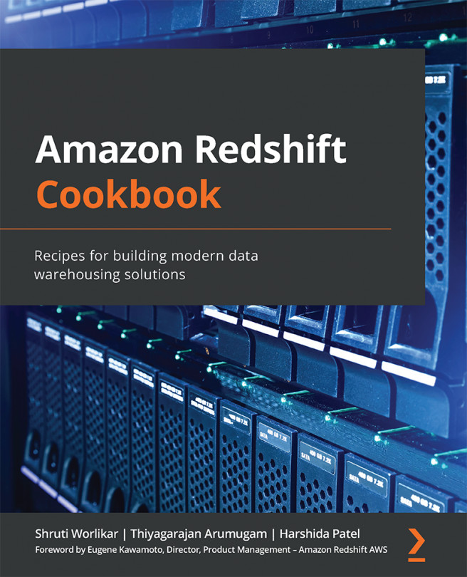
Amazon Redshift Cookbook

Amazon Redshift Cookbook: Recipes for building modern data warehousing solutions

By Shruti Worlikar , Thiyagarajan Arumugam , Harshida Patel
NZ$‎64.99 NZ$‎44.99
Book Jul 2021 384 pages 1st Edition
eBook
NZ$‎64.99 NZ$‎44.99
Print
NZ$‎80.99
Subscription
Free Trial
eBook
NZ$‎64.99 NZ$‎44.99
Print
NZ$‎80.99
Subscription
Free Trial

What do you get with eBook?

Product feature icon Instant access to your Digital eBook purchase
Product feature icon Download this book in EPUB and PDF formats
Product feature icon Access this title in our online reader with advanced features
Product feature icon DRM FREE - Read whenever, wherever and however you want
Buy Now

Product Details


Publication date : Jul 23, 2021
Length 384 pages
Edition : 1st Edition
Language : English
ISBN-13 : 9781800569683
Category :
Concepts :
Table of content icon View table of contents Preview book icon Preview Book

Amazon Redshift Cookbook

Chapter 2: Data Management

Amazon Redshift is a data warehousing service optimized for online analytical processing (OLAP) applications. You can start with just a few hundred gigabytes (GB) of data and scale to a petabyte (PB) or more. Designing your database for analytical processing lets you take full advantage of Amazon Redshift's columnar architecture.

An analytical schema forms the foundation of your data model. This chapter explores how you can set up this schema, thus enabling convenient querying using standard Structured Query Language (SQL) and easy administration of access controls.

The following recipes are discussed in this chapter:

  • Managing a database in an Amazon Redshift cluster
  • Managing a schema in a database
  • Managing tables
  • Managing views
  • Managing materialized views
  • Managing stored procedures
  • Managing user-defined functions (UDFs)

Technical requirements

In order to complete the recipes in this chapter, you will need a SQL client of your choice to access the Amazon Redshift cluster (for example, MySQL Workbench).

Managing a database in an Amazon Redshift cluster

Amazon Redshift consists of at least one database, and it is the highest level in the namespace hierarchy for the objects in the cluster. This recipe will guide you through the steps needed to create and manage a database in Amazon Redshift.

Getting ready

To complete this recipe, you will need the following:

  • Access to any SQL interface such as a SQL client or query editor
  • An Amazon Redshift cluster endpoint

How to do it…

Let's now set up and configure a database on the Amazon Redshift cluster. Use the SQL client to connect to the cluster and execute the following commands:

  1. We will create a new database called qa in the Amazon Redshift cluster. To do this, use the following code:
    CREATE DATABASE qa
    WITH 
    OWNER awsuser 
    CONNECTION LIMIT 50; 
  2. To view the details of the database, you will query the PG_DATABASE_INFO, as shown in the following code snippet:
    SELECT datname, datdba, datconnlimit 
    FROM pg_database_info
    WHERE datdba > 1;

    This is the expected output:

    datname datdba  datconnlimit
    qa 100 UNLIMITED

    This query will list the databases that exist in the cluster. If a database is successfully created, it will show up in the query result.

  3. To make changes to the database—such as database name, owner, and connection limit—use the following command, replacing <qauser> with the respective Amazon Redshift username:
    /* Change database owner */
    ALTER DATABASE qa owner to <qauser>;
    /* Change database connection limit */
    ALTER DATABASE qa CONNECTION LIMIT 100;
    /* Change database name */
    ALTER DATABASE qa RENAME TO prod;
  4. To verify that the changes have been successfully completed, you will query the system table pg_database_info, as shown in the following code snippet, to list all the databases in the cluster:
    SELECT datname, datdba, datconnlimit 
    FROM pg_database_info
    WHERE datdba > 1;

    This is the expected output:

    datname datdba datconnlimit
    prod 100 100
  5. You can connect to the prod database using the connection endpoint, as follows:
    <RedshiftClusterHostname>:<Port>/prod

    Here, prod refers to the database you would like to connect to.

  6. To delete the previously created database, execute the following query:
    DROP DATABASE prod;

    Important note

    It is best practice to have only one database in production per Amazon Redshift cluster. Multiple databases could be created in a development environment to enable separation of functions such a development/unit testing/quality assurance (QA). Within the same session, it is not possible to access objects across multiple databases, even though they are present in the same cluster. The only exception to this rule is database users and groups that are available across the databases.

Managing a schema in a database

In Amazon Redshift, a schema is a namespace that groups database objects such as tables, views, stored procedures, and so on. Organizing database objects in a schema is good for security monitoring and also logically groups the objects within a cluster. In this recipe, we will create a sample schema that will be used to hold all the database objects.

Getting ready

To complete this recipe, you will need access to any SQL interface such as a SQL client or query editor.

How to do it…

  1. Users can create a schema using the CREATE SCHEMA command. The following steps will enable you to set up a schema with the name finance and add the necessary access to the groups.
  2. Create finance_grp, audit_grp, and finance_admin_user groups using the following command:
    create group finance_grp;
    create group audit_grp;
    create user finance_admin_usr with password '<PasswordOfYourChoice>'; 
  3. Create a schema named finance with a space quota of 2 terabytes (TB), with a finance_admin_usr schema owner:
    CREATE schema finance authorization finance_admin_usr QUOTA 2 TB;

    You can also modify an existing schema using ALTER SCHEMA or DROP SCHEMA.

  4. For the finance schema, grant access privileges of USAGE and ALL to the finance_grp group. Further, grant read access to the tables in the schema using a SELECT privilege for the audit_grp group:
    GRANT USAGE on SCHEMA finance TO GROUP finance_grp;
    GRANT USAGE on SCHEMA finance TO GROUP audit_grp;
    GRANT ALL ON schema finance to GROUP finance_grp;
    GRANT SELECT ON ALL TABLES IN SCHEMA finance TO GROUP audit_grp;
  5. You can verify that the schema and owner group have been created by using the following code:
    select nspname as schema, usename as owner
    from pg_namespace, pg_user
    where pg_namespace.nspowner = pg_user.usesysid
    and pg_namespace.nspname ='finance';
  6. Create a foo table (or view/database object) within the schema by prefixing the schema name along with the table name, as shown in the following command:
    CREATE TABLE finance.foo (bar int); 
  7. Now, in order to select the foo table from the finance schema, you will have to prefix the schema name along with the table name, as shown in the following command:
    select * from finance.foo; 

    The preceding SQL code will not return any rows.

  8. Assign a search path to conveniently reference the database objects directly, without requiring the complete namespace of the schema qualifier. The following command sets the search path as finance so that you don't need to qualify the schema name every time when working with database objects:
    set search_path to '$user', finance, public;

    Important note

    The search path allows a convenient way to access the database objects without having to specify the target schema in the namespace when authoring the SQL code. The search path can be configured using the search_path parameter with a comma-separated list of schema names. When referencing the database object in a SQL when no target schema is provided, the database object that is in the first available schema list is picked up. You can configure the search path by using the SET search_path command at the current session level or at the user level.

  9. Now, executing the following SELECT query without the schema qualifier automatically locates the foo table in the finance schema:
    select * from foo;

    The preceding SQL code will not return any rows.

Now, the new finance schema is ready for use and you can keep creating new database objects in this schema.

Important note

A database is automatically created by default with a PUBLIC schema. Identical database object names can be used in different schemas of the database. For example, finance.customer and marketing.customer are valid table definitions that can be created without any conflict, where finance and marketing are schema names and customer is the table name. Schemas serve the key purpose of easy management through this logical grouping—for example, you can grant SELECT access to all the objects at a schema level instead of individual tables.

Managing tables

In Amazon Redshift, you can create a collection of tables within a schema with related entities and attributes. Working backward from your business requirements, you can use different modeling techniques to create tables in Amazon Redshift. You can choose a star or snowflake schema by using Normalized, Denormalized, or Data Vault data modeling techniques.

In this recipe, we will create tables in the finance schema, insert data into those tables and cover the key concepts to leverage the massively parallel processing (MPP) and columnar architecture.

Getting ready

To complete this recipe you will need a SQL client, or you can use the Amazon Redshift query editor.

How to do it…

Let's explore how to create tables in Amazon Redshift.

  1. Let's create a customer table in the finance schema with customer_number, first_name, last_name, and date_of_birth related attributes:
    CREATE TABLE finance.customer 
    (
      customer_number   INTEGER,
      first_name        VARCHAR(50),
      last_name         VARCHAR(50),
      date_of_birth     DATE
    );

    Note

    The key ingredient when creating a customer table is to define columns and their corresponding data types. Amazon Redshift supports data types such as numeric, character, date, datetime with time zone, boolean, geometry, HyperLogLog, and super.

  2. We will now insert 10 records into the customer table using a multi-value insert statement:
    insert into finance.customer values
    (1, 'foo', 'bar', '1980-01-01'),
    (2, 'john', 'smith', '1990-12-01'),
     (3, 'spock', 'spock', '1970-12-01'),
     (4, 'scotty', 'scotty', '1975-02-01'),
     (5, 'seven', 'of nine', '1990-04-01'),
     (6, 'kathryn', 'janeway', '1995-07-01'),
     (7, 'tuvok', 'tuvok', '1960-06-10'),
     (8, 'john', 'smith', '1965-12-01'),
     (9, 'The Doctor', 'The Doctor', '1979-12-01'),
     (10, 'B Elana', 'Torres', '2000-08-01');
  3. You can now review the information on the customer table using the svv_table_info system view. Execute the following query:
    select "schema", table_id, "table", encoded, diststyle, sortkey1,  size, tbl_rows
    from svv_Table_info
    where "table" = 'customer'
    and "schema" = 'finance';

    This is the expected output:

    schema table_id table encoded diststyle sortkey1 size tbl_rows
    finance 167482 customer Y AUTO(ALL) AUTO(SORTKEY) 14 10

    Table_id is the object ID and the number of records in the table is 10 rows. The encoded column indicates the table is compressed. Amazon Redshift stores columns in 1 megabyte (MB) immutable blocks. The size of the table is 14 MB. Let's dive into the terminology and concept of diststyle and sortkey. The customer table is created with default sort key of AUTO, where Amazon Redshift handles the distribution style of the table on the computer nodes.

    • diststyle is a table property that dictates how that table's data is distributed throughout the cluster.
    • KEY: The value is hashed, and the same value goes to same location (slice) on the compute node.
    • ALL: The full table data goes to the first slice of every compute node.
    • EVEN: Round-robin across all the compute nodes.
    • AUTO: When the table is small, it starts with an AUTO style, and when it becomes larger in size, Amazon Redshift converts it to an EVEN style.

Further information about distribution styles can be found at the following link:

https://docs.aws.amazon.com/redshift/latest/dg/c_choosing_dist_sort.html

  1. Let's run a query against the customer table to list customers who were born before 1980:
    select *
    from finance.customer
    where extract(year from date_of_birth) < 1980;
  2. You can also create a copy of the permanent table using create table as (CTAS). Let's execute the following query to create another table for a customer born in 1980:
    create table finance.customer_dob_1980 as 
    select *
    from finance.customer
    where extract(year from date_of_birth) = 1980 ;
  3. You can also create temporary tables—for example, to generate IDs in a data loading operation. The temporary tables can only be queried during the current session and are automatically dropped when the session ends. The temporary tables are created in the session-specific schema and are not visible to any other user. You can use a create temporary table command to do this. Execute the following three queries in single session:
    create temporary table #customer(custid integer IDENTITY(1,1), customer_number integer);
    insert into #customer (customer_number) values(1);
    select * from #customer;

    This is the expected output:

    custid  customer_number
    1 1
  4. Reconnect to the Amazon Redshift cluster using the SQL client. Reconnecting will create a new session. Now, try to execute the following query against the #customer temporary table. You will get an ERROR: 42P01: relation "#customer" does not exist error message as the temporary tables are only visible to the current session:
    select * from #customer;

How it works…

When you create a table in Amazon Redshift, it stores the data on disk, column by column, on 1 MB blocks. Amazon Redshift by default compresses the columns, which reduces the storage footprint and the input/output (I/O) when you execute a query against the table. Amazon Redshift provides different distribution styles to spread the data across all the compute nodes, to leverage the MPP architecture for your workload. The metadata and the table summary information can be queried using the catalog table and summary view.

Amazon Redshift stores metadata about the customer table. You can query the pg_table_def catalog table to retrieve this information. You can execute the following query to view the table/column structure:

select * from pg_table_def where schemaname = 'finance';. 

Important note

When data is inserted into a table, Amazon Redshift automatically builds, in memory, the metadata of the minimum and maximum values of each block. This metadata, known as a zone map, is accessed before a disk scan in order to identify which blocks are relevant to a query. Amazon Redshift does not have indexes; it does, however, have sort keys. Sort key columns govern how data is physically sorted for a table on disk and can be used as a lever to improve query performance. Sort keys will be covered in depth in the performance-tuning best practices chapter.

Managing views

View database objects allow the result of a query to be stored. In Amazon Redshift, views run each time a view is mentioned in a query. The advantage of using a view instead of a table is that it can allow access to only a subset of data on a table, join more than one table in a single virtual table, and act as an aggregated table, and it takes up no space on the database since only the definition is saved, hence making it convenient to abstract complicated queries. In this recipe, we will create views to store queries for the underlying tables.

Getting ready

To complete this recipe, you will need access to any SQL interface such as a SQL client or query editor.

How to do it…

Let's create a view using the CREATE VIEW command. We will use the following steps to create a view:

  1. Create a finance.customer_vw view based on the results of the query on finance.customer:
    CREATE VIEW finance.customer_vw 
    AS
    SELECT customer_number,
           first_name,
           last_name,
           EXTRACT(year FROM date_of_birth) AS year_of_birth
    FROM finance.customer;
  2. To verify that a view has been created, you can use the following command:
    SELECT table_schema as schema_name,
           table_name as view_name,
           view_definition
    FROM information_schema.views
    WHERE table_schema not in ('information_schema', 'pg_catalog')
    ORDER by schema_name,
             view_name;

    Note

    This script will provide an output of the views created under a particular schema and the SQL script for the view.

  3. We can now select directly from the finance.customer_vw view, just like with any another database object, like so:
    SELECT * from finance.customer_vw limit 5;

    Note

    Here, the finance.customer_vw view abstracts the date_of_birth personally identifiable information (PII) from the underlying table and provides the user an abstracted view of only the essential data for that year to determine the age group.

    This is the expected output:

    outputcustomer_number,first_name,last_name,year_of_birth 
    1 foo bar 1980
    2 john smith 1990
    3 spock spock 1970
    4 scotty scotty 1975
    5 seven of nine 1990 
  4. To delete the previously created view, you can use the following command:
    DROP VIEW finance.customer_vw ;

Managing materialized views

A materialized view is a database object that persists the results of a query to disk. In Amazon Redshift, materialized views allow frequently used complex queries to be stored as separate database objects, allowing you to access these database objects directly, and enabling faster query responses.

Employing materialized views is a common approach to powering repeatable queries in a business intelligence (BI) dashboard, and avoids expensive computation each time. Furthermore, materialized views allow an incremental refresh of the results, using the underlying table data. In this recipe, we will create a materialized view to query the tables and also to persist the results to fetch the data more quickly.

Getting ready

To complete this recipe, you will need access to any SQL interface such as a SQL client or a query editor.

How to do it…

Let's create a materialized view using the CREATE MATERIALIZED VIEW command. We will use the following steps to create a materialized view, in order to store the precomputed results of an analytical query and also see how to refresh it:

  1. Create a finance.customer_agg_mv materialized view using the results of the query based on finance.customer:
    CREATE MATERIALIZED VIEW finance.customer_agg_mv
    AS
    SELECT 
           EXTRACT(year FROM date_of_birth) AS year_of_birth,
           count(1) customer_cnt
    FROM finance.customer
    group by EXTRACT(year FROM date_of_birth);
  2. We can now select directly from finance.customer, just like with any another database object, like so:
    select * from finance.customer limit 5;

    This is the expected output:

    outputyear_of_birth,customer_cnt 
    1975 1
    1979 1
    1995 1
    1970 1
    1965 1
  3. You can verify the state of a materialized view by using a STV_MV_INFO system table (https://docs.aws.amazon.com/redshift/latest/dg/r_STV_MV_INFO.html):
    select * from STV_MV_INFO where name='customer_agg_mv';

    This is the expected output:

    outputdb_name,schema,name,updated_upto_xid,is_stale,owner_user_name,state,autorefresh, autorewrite
    vdwpoc  finance customer_agg_mv 24642401 f vdwadmin 1 f t

    Here, stale='f' indicates the data is current, reflecting the daily_product_reviews underlying base table. This column can be used to refresh the materialized view when needed. Another key column in the STV_MV_INFO table is the state column, which indicates if an incremental refresh is possible (state=1) or not (state=0). In the materialized view we created a state=1 state, which indicates a faster incremental refresh is possible.

  4. Now, let's load more data into the underlying table finance.customer, using the following command, and check the STV_MV_INFO table:
    insert into finance.customer values
    (11, 'mark', 'bar', '1980-02-01'),
    (12, 'pete', 'smith', '1990-2-01'),
     (13, 'woofy', 'spock', '1980-11-01'),
     (14, 'woofy jr', 'scotty', '1975-03-01'),
     (15, 'eleven', 'of nine', '1990-07-01');
  5. Query the STV_MV_INFO table again to check the status of the materialized view:
    select name,is_stale,state from STV_MV_INFO where name='customer_agg_mv'; 

    This is the expected output:

    name,is_stale,state
    customer_agg_mv
    t 1

    Note that stale = 't' indicates that the underlying data for the materialized view has changed, but it is possible to refresh it incrementally.

  6. Refresh the materialized view using the REFRESH MATERIALIZED VIEW command and check the status again:
    REFRESH MATERIALIZED VIEW finance.customer_agg_mv;
    select name,is_stale, state from STV_MV_INFO where name='customer_agg_mv';

    This is the expected output:

    name,is_stale,state
    customer_agg_mv  f 1

    As we can see from the preceding code snippet, customer_agg_mv is now updated to reflect the underlying table data.

How it works…

A materialized view can be updated with the latest data from the underlying tables by using the REFRESH MATERIALIZED VIEW command. When the materialized view is being refreshed, it executes a separate transaction to update the dataset. Amazon Redshift also supports an autorefresh option to keep the materialized view up to date as soon as possible after base tables change.

Managing stored procedures

Stored procedures in Amazon Redshift are user-created objects using a Procedural Language/PostgreSQL (PL/pgSQL) procedural programming language. Stored procedures support both data definition language (DDL) and data manipulation language (DML). Stored procedures can take in input arguments but do not necessarily need to return results. PL/pgSQL also supports conditional logic, loops, and case statements. Stored procedures are commonly used to build reusable extract, transform, load (ETL) data pipelines and enable the database administrator (DBA) to automate routine administrative activities—for example, periodically dropping unused tables.

The SECURITY attribute controls who has privileges to access certain database objects.

Stored procedures can be created with security definer controls to allow execution of a procedure without giving access to underlying tables—for example, they can drop a table created by another user and enable the DBA to automate administrative activities.

Getting ready

To complete this recipe, you will need the following:

  • Access to the Amazon Web Services (AWS) Management Console
  • Access to any SQL interface such as a SQL client or query editor

How to do it…

In this recipe, we will start with creating a scalar Python-based UDF that will be used to parse an Extensible Markup Language (XML) input:

  1. Connect to Amazon Redshift using the SQL client, and copy and paste the following code to create a sp_cookbook stored procedure:
    Create schema cookbook;
    create or replace procedure sp_cookbook(indate in date, records_out INOUT refcursor) as
    $$
    declare
      integer_var int;
    begin
       RAISE INFO 'running first cookbook storedprocedure on date %',  indate;
       drop table if exists cookbook.cookbook_tbl;
      create table cookbook.cookbook_tbl
      (recipe_name varchar(50),
       recipe_date date
       );
       insert into cookbook.cookbook_tbl values('stored procedure', indate);
      GET DIAGNOSTICS integer_var := ROW_COUNT;
       RAISE INFO 'rows inserted into cookbook_tbl = %', integer_var;
        OPEN records_out FOR SELECT * FROM cookbook.cookbook_tbl;
    END;   
    $$ LANGUAGE plpgsql;

    This stored procedure is taking two parameters: indate is the input, and records_out serves as both an input and output parameter. This stored procedure uses DDL and DML statements. The current user is the owner of the stored procedure and is also the owner of the cookbook.cookbook_tbl table.

    Note

    Some older versions of SQL client tools may produce an "unterminated dollar-quoted string at or near "$$"error. Ensure that you have the latest version of the SQL client—for example, ensure you are using version 124 or higher for the SQL Workbench/J client.

  2. Now, let's execute the sp_cookbook stored procedure using the following statements:
    call sp_cookbook(current_date, 'inputcursor');
    fetch all from inputcursor;

    This is the expected output:

    Message
    running first cookbook storedprocedure on date 2020-12-13
    rows inserted into cookbook_tbl = 1
    recipe_name recipe_date
    stored procedure   2020-12-13 00:00:00
  3. To view a definition of the previously created stored procedure, you can run the following statement:
    SHOW PROCEDURE sp_cookbook(indate in date, records_out INOUT refcursor);
  4. We will now create another stored procedure with a security definer privilege:
    create or replace procedure public.sp_self_service(tblName in varchar(60)) as
                $$ 
    begin        
        RAISE INFO 'running sp_self_service to drop table %',  tblName;
        execute 'drop table if exists cookbook.' || tblName;
      RAISE INFO 'table dropped %',  tblName;
    END;   
    $$ LANGUAGE plpgsql
    SECURITY DEFINER;
  5. Let's create a user and check whether they have a permission to drop the cookbook.cookbook_tbl table. The user1 user does not have a permission to drop the table:
    create user user1 with password 'Cookbook1';
    grant execute on procedure public.sp_self_service(tblName in varchar(60)) to user1;
    set SESSION authorization  user1;
    select current_user;
    drop table cookbook.cookbook_tbl;

    This is the expected output:

    ERROR: 42501: permission denied for schema cookbook
  6. When user1 executes the sp_self_service stored procedure, the procedure runs with the security context of the owner of the procedure:
    set SESSION authorization  user1;
    select current_user;
    call public.sp_self_service('cookbook_tbl');

    This is the expected output:

    running sp_self_service to drop table cookbook_tbl
    table 

    This allows the user to drop the table without providing the full permissions for the tables in the cookbook schema.

How it works…

Amazon Redshift uses the PL/pgSQL procedural language for authoring the stored procedures. PL/pgSQL provides programmatic access that can be used to author control structures to the SQL language and allow complex computations. For example, you have a stored procedure that can create users and set up necessary access that meets your organizational needs—hence, rather than invoking several commands, this can now be done in a single step. You can find the complete reference to the PL/pgSQL procedural language at https://www.postgresql.org/docs/8.0/plpgsql.html and ready-to-use stored useful procedures at https://github.com/awslabs/amazon-redshift-utils/tree/master/src/StoredProcedures. The SECURITY access attribute of a stored procedure defines the privileges to access underlying database objects used. By default, an INVOKER is used to access the user privileges and the SECURITY DEFINER allows the procedure user to inherit the privileges of the owner.

Managing UDFs

Scalar UDF functions in Amazon Redshift are routines that are able to take parameters, perform calculations, and return the results. UDFs are handy when performing complex calculations that can be stored and reused in a SQL statement. Amazon Redshift supports UDFs that can be authored using either Python or SQL. In addition, Amazon Redshift also supports AWS Lambda UDFs that open up further possibilities to invoke other AWS services. For example, let's say the latest customer address information is stored in AWS DynamoDB—you can invoke an AWS Lambda UDF to retrieve this using a SQL statement in Amazon Redshift.

Getting ready

To complete this recipe, you will need the following:

  • Access to the AWS console
  • Access to any SQL interface such as a SQL client or query editor
  • Access to create an AWS Lambda function
  • Access to create an Identity and Access Management (IAM) role that can invoke AWS Lambda and attach it to Amazon Redshift

How to do it…

In this recipe, we will start with a scalar Python-based UDF that will be used to parse an XML input:

  1. Connect to Amazon Redshift using the SQL client, and copy and paste the following code to create an f_parse_xml function:
    CREATE OR REPLACE FUNCTION f_parse_xml
    (xml VARCHAR(MAX), input_rank int)
    RETURNS varchar(max)
    STABLE
    AS $$
        import xml.etree.ElementTree as ET
        root = ET.fromstring(xml)
        res = ''
        for country in root.findall('country'):
            rank = country.find('rank').text
            if rank == input_rank:
               res =  name = country.get('name') + ':' + rank
               break
        return res 
    $$ LANGUAGE plpythonu;

    Important note

    The preceding Python-based UDF takes in the XML data and uses the xml.etree.ElementTree library to parse it to locate an element, using the input rank. See https://docs.python.org/3/library/xml.etree.elementtree.html for more options that are available with this XML library.

  2. Now, let's validate the f_parse_xml function using the following statement, by locating the country name that has the rank 2:
    select 
    f_parse_xml('<data>      <country name="Liechtenstein">        <rank>2</rank>         <year>2008</year>         <gdppc>141100</gdppc>         <neighbor name="Austria" direction="E"/>        <neighbor name="Switzerland" direction="W"/> </country></data>', '2') as col1

    This is the expected output:

    col1
    Liechtenstein:2
  3. We will now create another AWS Lambda-based UDF. Navigate to the AWS Management Console and pick the AWS Lambda service and click on Create function, as shown in the following screenshot:
    Figure 2.1 – Creating a Lambda function using the AWS Management Console

    Figure 2.1 – Creating a Lambda function using the AWS Management Console

  4. In the Create function screen, enter rs_lambda under Function name, choose a Python 3.6 runtime, and click on Create function.
  5. Under the Function code textbox, copy and paste the following code and press the Deploy button:
    import json
    def lambda_handler(event, context):
        ret = dict()
        ret['success'] = True
        ret['results'] = ["bar"]
        ret['error_msg'] = "none"
        ret['num_records'] = 1
        return json.dumps(ret)

    In the preceding Python-based Lambda function, a sample result is returned. This function can further be integrated to call any other AWS service—for example, you can invoke AWS Key Management Service (KMS) to encrypt input data.

  6. Navigate to AWS IAM in the AWS Management Console and create a new role, RSInvokeLambda, using the following policy statement by replacing [Your_AWS_Account_Number], [Your_AWS_Region] with your AWS account number/region and attaching the role to the Amazon Redshift cluster:
    {
        "Version": "2012-10-17",
        "Statement": [
            {
                "Effect": "Allow",
                "Action": "lambda:InvokeFunction",
                "Resource": "arn:aws:lambda:[Your_AWS_Region]: [Your_AWS_Account_Number]:function:rs_lambda"
            }
        ]
    }
  7. Connect to Amazon Redshift using the SQL client, and copy and paste the following code to create a f_redshift_lambda function that links the AWS Lambda rs_lambda function:
    CREATE OR REPLACE EXTERNAL FUNCTION f_redshift_lambda (bar varchar)
    RETURNS varchar STABLE
    LAMBDA 'rs_lambda'
    IAM_ROLE 'arn:aws:iam::[Your_AWS_Account_Number]:role/RSInvokeLambda';
  8. You can validate the f_redshift_lambda function by using the following SQL statement:
    select f_redshift_lambda ('input_str') as col1
    --output
    col1
    bar

Amazon Redshift is now able to invoke the AWS Lambda function using a SQL statement.

How it works…

Amazon Redshift allows you to create a scalar UDF using either a SQL SELECT clause or a Python program in addition to the AWS Lambda UDF illustrated in this recipe. The scalar UDFs are stored with Amazon Redshift and are available to any user when granted the required access. You can find a collection of several ready-to-use UDFs that can be used to implement some of the complex reusable logic within a SQL statement at the following link: https://github.com/aws-samples/amazon-redshift-udfs.

Left arrow icon Right arrow icon
Download code icon Download Code

Key benefits

  • Discover how to translate familiar data warehousing concepts into Redshift implementation
  • Use impressive Redshift features to optimize development, productionizing, and operations processes
  • Find out how to use advanced features such as concurrency scaling, Redshift Spectrum, and federated queries

Description

Amazon Redshift is a fully managed, petabyte-scale AWS cloud data warehousing service. It enables you to build new data warehouse workloads on AWS and migrate on-premises traditional data warehousing platforms to Redshift. This book on Amazon Redshift starts by focusing on Redshift architecture, showing you how to perform database administration tasks on Redshift. You'll then learn how to optimize your data warehouse to quickly execute complex analytic queries against very large datasets. Because of the massive amount of data involved in data warehousing, designing your database for analytical processing lets you take full advantage of Redshift's columnar architecture and managed services. As you advance, you’ll discover how to deploy fully automated and highly scalable extract, transform, and load (ETL) processes, which help minimize the operational efforts that you have to invest in managing regular ETL pipelines and ensure the timely and accurate refreshing of your data warehouse. Finally, you'll gain a clear understanding of Redshift use cases, data ingestion, data management, security, and scaling so that you can build a scalable data warehouse platform. By the end of this Redshift book, you'll be able to implement a Redshift-based data analytics solution and have understood the best practice solutions to commonly faced problems.

What you will learn

Use Amazon Redshift to build petabyte-scale data warehouses that are agile at scale Integrate your data warehousing solution with a data lake using purpose-built features and services on AWS Build end-to-end analytical solutions from data sourcing to consumption with the help of useful recipes Leverage Redshift s comprehensive security capabilities to meet the most demanding business requirements Focus on architectural insights and rationale when using analytical recipes Discover best practices for working with big data to operate a fully managed solution

What do you get with eBook?

Product feature icon Instant access to your Digital eBook purchase
Product feature icon Download this book in EPUB and PDF formats
Product feature icon Access this title in our online reader with advanced features
Product feature icon DRM FREE - Read whenever, wherever and however you want
Buy Now

Product Details


Publication date : Jul 23, 2021
Length 384 pages
Edition : 1st Edition
Language : English
ISBN-13 : 9781800569683
Category :
Concepts :

Table of Contents

13 Chapters
Preface Chevron down icon Chevron up icon
Chapter 1: Getting Started with Amazon Redshift Chevron down icon Chevron up icon
Chapter 2: Data Management Chevron down icon Chevron up icon
Chapter 3: Loading and Unloading Data Chevron down icon Chevron up icon
Chapter 4: Data Pipelines Chevron down icon Chevron up icon
Chapter 5: Scalable Data Orchestration for Automation Chevron down icon Chevron up icon
Chapter 6: Data Authorization and Security Chevron down icon Chevron up icon
Chapter 7: Performance Optimization Chevron down icon Chevron up icon
Chapter 8: Cost Optimization Chevron down icon Chevron up icon
Chapter 9: Lake House Architecture Chevron down icon Chevron up icon
Chapter 10: Extending Redshift's Capabilities Chevron down icon Chevron up icon
Other Books You May Enjoy Chevron down icon Chevron up icon
Appendix Chevron down icon Chevron up icon

Customer reviews

Filter icon Filter
Top Reviews
Rating distribution
Empty star icon Empty star icon Empty star icon Empty star icon Empty star icon 0
(0 Ratings)
5 star 0%
4 star 0%
3 star 0%
2 star 0%
1 star 0%

Filter reviews by


No reviews found
Get free access to Packt library with over 7500+ books and video courses for 7 days!
Start Free Trial

FAQs

How do I buy and download an eBook? Chevron down icon Chevron up icon

Where there is an eBook version of a title available, you can buy it from the book details for that title. Add either the standalone eBook or the eBook and print book bundle to your shopping cart. Your eBook will show in your cart as a product on its own. After completing checkout and payment in the normal way, you will receive your receipt on the screen containing a link to a personalised PDF download file. This link will remain active for 30 days. You can download backup copies of the file by logging in to your account at any time.

If you already have Adobe reader installed, then clicking on the link will download and open the PDF file directly. If you don't, then save the PDF file on your machine and download the Reader to view it.

Please Note: Packt eBooks are non-returnable and non-refundable.

Packt eBook and Licensing When you buy an eBook from Packt Publishing, completing your purchase means you accept the terms of our licence agreement. Please read the full text of the agreement. In it we have tried to balance the need for the ebook to be usable for you the reader with our needs to protect the rights of us as Publishers and of our authors. In summary, the agreement says:

  • You may make copies of your eBook for your own use onto any machine
  • You may not pass copies of the eBook on to anyone else
How can I make a purchase on your website? Chevron down icon Chevron up icon

If you want to purchase a video course, eBook or Bundle (Print+eBook) please follow below steps:

  1. Register on our website using your email address and the password.
  2. Search for the title by name or ISBN using the search option.
  3. Select the title you want to purchase.
  4. Choose the format you wish to purchase the title in; if you order the Print Book, you get a free eBook copy of the same title. 
  5. Proceed with the checkout process (payment to be made using Credit Card, Debit Cart, or PayPal)
Where can I access support around an eBook? Chevron down icon Chevron up icon
  • If you experience a problem with using or installing Adobe Reader, the contact Adobe directly.
  • To view the errata for the book, see www.packtpub.com/support and view the pages for the title you have.
  • To view your account details or to download a new copy of the book go to www.packtpub.com/account
  • To contact us directly if a problem is not resolved, use www.packtpub.com/contact-us
What eBook formats do Packt support? Chevron down icon Chevron up icon

Our eBooks are currently available in a variety of formats such as PDF and ePubs. In the future, this may well change with trends and development in technology, but please note that our PDFs are not Adobe eBook Reader format, which has greater restrictions on security.

You will need to use Adobe Reader v9 or later in order to read Packt's PDF eBooks.

What are the benefits of eBooks? Chevron down icon Chevron up icon
  • You can get the information you need immediately
  • You can easily take them with you on a laptop
  • You can download them an unlimited number of times
  • You can print them out
  • They are copy-paste enabled
  • They are searchable
  • There is no password protection
  • They are lower price than print
  • They save resources and space
What is an eBook? Chevron down icon Chevron up icon

Packt eBooks are a complete electronic version of the print edition, available in PDF and ePub formats. Every piece of content down to the page numbering is the same. Because we save the costs of printing and shipping the book to you, we are able to offer eBooks at a lower cost than print editions.

When you have purchased an eBook, simply login to your account and click on the link in Your Download Area. We recommend you saving the file to your hard drive before opening it.

For optimal viewing of our eBooks, we recommend you download and install the free Adobe Reader version 9.