Search icon CANCEL
Subscription
0
Cart icon
Cart
Close icon
You have no products in your basket yet
Save more on your purchases!
Savings automatically calculated. No voucher code required
Arrow left icon
All Products
Best Sellers
New Releases
Books
Videos
Audiobooks
Learning Hub
Newsletters
Free Learning
Arrow right icon
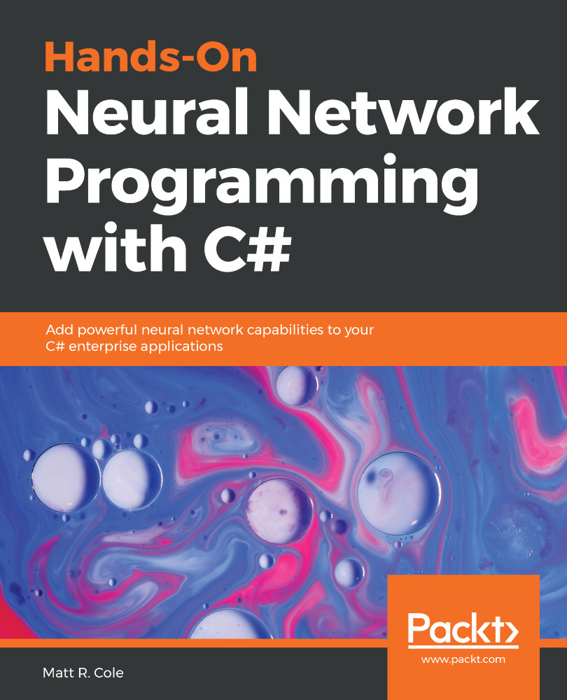
Hands-On Neural Network Programming with C#

Hands-On Neural Network Programming with C#: Add powerful neural network capabilities to your C# enterprise applications

Profile Icon Matt Cole
By Matt Cole
$24.99 $35.99
Book Sep 2018 328 pages 1st Edition
eBook
$24.99 $35.99
Print
$43.99
Subscription
Free Trial
Renews at $19.99p/m
Profile Icon Matt Cole
By Matt Cole
$24.99 $35.99
Book Sep 2018 328 pages 1st Edition
eBook
$24.99 $35.99
Print
$43.99
Subscription
Free Trial
Renews at $19.99p/m
eBook
$24.99 $35.99
Print
$43.99
Subscription
Free Trial
Renews at $19.99p/m

What do you get with eBook?

Product feature icon Instant access to your Digital eBook purchase
Product feature icon Download this book in EPUB and PDF formats
Product feature icon Access this title in our online reader with advanced features
Product feature icon DRM FREE - Read whenever, wherever and however you want
Table of content icon View table of contents Preview book icon Preview Book

Hands-On Neural Network Programming with C#

A Quick Refresher

Welcome to Hands-On Neural Network Development Using C#. I want to thank you for purchasing this book and for taking this journey with us. It seems as if, everywhere you turn, everywhere you go, all you hear and read about is machine learning, artificial intelligence, deep learning, neuron this, artificial that, and on and on. And, to add to all that excitement, everyone you talk to has a slightly different idea about the meaning of each of those terms.

In this chapter, we are going to go over some very basic neural network terminology to set the stage for future chapters. We need to be speaking the same language, just to make sure that everything we do in later chapters is crystal clear.

I should also let you know that the goal of the book is to get you, a C# developer, up and running as fast as possible. To do this, we will use as many open source libraries as possible. We must do a few custom applications, but we've provided the source code for these as well. In all cases, we want you to be able to add this functionality to your applications with maximal speed and minimal effort.

OK, let's begin.

Neural networks have been around for very many years but have made a resurgence over the past few years and are now a hot topic. And that, my friends, is why this book is being written. The goal here is to help you get through the weeds and into the open so you can navigate your neural path to success. There is a specific focus in this book on C# .NET developers. I wanted to make sure that the C# developers out there had handy resources that could be of some help in their projects, rather than the Python, R, and MATLAB code we more commonly see. If you have Visual Studio installed and a strong desire to learn, you are ready to begin your journey.

First, let's make sure we're clear on a couple of things. In writing this book, the assumption was made that you, the reader, had limited exposure to neural networks. If you do have some exposure, that is great; you may feel free to jump to the sections that interest you the most. I also assumed that you are an experienced C# developer, and have built applications using C#, .NET, and Visual Studio, although I made no assumptions as to which versions of each you may have used. The goal is not about C# syntax, the .NET framework, or Visual Studio itself. Once again, the purpose is to get as many valuable resources into the hands of developers, so they can embellish their code and create world-class applications.

Now that we've gotten that out of the way, I know you're excited to jump right in and start coding, but to make you productive, we first must spend some time going over some basics. A little bit of theory, some fascinating insights into the whys and wherefores, and we're going to throw in a few visuals along the way to help with the rough-and-tough dry stuff. Don't worry; we won't go too deep on the theory, and, in a few pages from here, you'll be writing and going through source code!

Also, keep in mind that research in this area is rapidly evolving. What is the latest and greatest today is old news next month. Therefore, consider this book an overview of different research and opinions. It is not the be-all-and-end-all bible of everything neural network-related, nor should it be perceived to be. You are very likely to encounter someone else with different opinions from that of the writer. You're going to find people who will write apps and functions differently. That's great—gather all the information that you can, and make informed choices on your own. Only doing by that will you increase your knowledge base.

This chapter will include the following topics:

  • Neural network overview
  • The role of neural networks in today's enterprises
  • Types of learning
  • Understanding perceptions
  • Understanding activation functions
  • Understanding back propagation

Technical requirements

Basic knowledge of C# is a must to understand the applications that we will develop in this book. Also, Microsoft Visual Studio (Any version) is a preferred software to develop applications.

Neural network overview

Let's start by defining exactly what we are going to call a neural network. Let me first note that you may also hear a neural network called an Artificial Neural Network (ANN). Although personally I do not like the term artificial, we'll use those terms interchangeably throughout this book.

"Let's state that a neural network, in its simplest form, is a system comprising several simple but highly interconnected elements; each processes information based upon their response to external inputs."

Did you know that neural networks are more commonly, but loosely, modeled after the cerebral cortex of a mammalian brain? Why didn't I say that they were modeled after humans? Because there are many instances where biological and computational studies are used from brains from rats, monkeys, and, yes, humans. A large neural network may have hundreds or maybe even thousands of processing units, where as a mammalian brain has billions. It's the neurons that do the magic, and we could in fact write an entire book on that topic alone.

Here's why I say they do all the magic: If I showed you a picture of Halle Berry, you would recognize her right away. You wouldn't have time to analyze things; you would know based upon a lifetime of collected knowledge. Similarly, if I said the word pizza to you, you would have an immediate mental image and possibly even start to get hungry. How did all that happen just like that? Neurons! Even though the neural networks of today continue to gain in power and speed, they pale in comparison to the ultimate neural network of all time, the human brain. There is so much we do not yet know or understand about this neural network; just wait and see what neural networks will become once we do!

Neural networks are organized into layers made up of what are called nodes or neurons. These nodes are the neurons themselves and are interconnected (throughout this book we use the terms nodes and neurons interchangeably). Information is presented to the input layer, processed by one or more hidden layers, then given to the output layer for final (or continued further) processing—lather, rinse, repeat!

But what is a neuron, you ask? Using the following diagram, let's state this:

"A neuron is the basic unit of computation in a neural network"

As I mentioned earlier, a neuron is sometimes also referred to as a node or a unit. It receives input from other nodes or external sources and computes an output. Each input has an associated weight (w1 and w2 below), which is assigned based on its relative importance to the other inputs. The node applies a function f (an activation function, which we will learn more about later on) to the weighted sum of its inputs. Although that is an extreme oversimplification of what a neuron is and what it can do, that's basically it.

Let's look visually at the progression from a single neuron into a very deep learning network. Here is what a single neuron looks like visually based on our description:

Next, the following diagram shows a very simple neural network comprised of several neurons:

Here is a somewhat more complicated, or deeper, network:

Neural network training

Now that we know what a neural network and neurons are, we should talk about what they do and how they do it. How does a neural network learn? Those of you with children already know the answer to this one. If you want your child to learn what a cat is, what do you do? You show them cats (pictures or real). You want your child to learn what a dog is? Show them dogs. A neural network is conceptually no different. It has a form of learning rule that will modify the incoming weights from the input layer, process them through the hidden layers, put them through an activation function, and hopefully will be able to identify, in our case, cats and dogs. And, if done correctly, the cat does not become a dog!

One of the most common learning rules with neural networks is what is known as the delta rule. This is a supervised rule that is invoked each time the network is presented with another learning pattern. Each time this happens it is called a cycle or epoch. The invocation of the rule will happen each time that input pattern goes through one or more forward propagation layers, and then through one or more backward propagation layers.

More simply put, when a neural network is presented with an image it tries to determine what the answer might be. The difference between the correct answer and our guess is the error or error rate. Our objective is that the error rate gets either minimized or maximized. In the case of minimization, we need the error rate to be as close to 0 as possible for each guess. The closer we are to 0, the closer we are to success.

As we progress, we undertake what is termed a gradient descent, meaning we continue along toward what is called the global minimum, our lowest possible error, which hopefully is paramount to success. We descend toward the global minimum.

Once the network itself is trained, and you are happy, the training cycle can be put to bed and you can move on to the testing cycle. During the testing cycle, only the forward propagation layer is used. The output of this process results in the model that will be used for further analysis. Again, no back propagation occurs during testing.

A visual guide to neural networks

In this section, I could type thousands of words trying to describe all of the combinations of neural networks and what they look like. However, no amount of words would do any better than the diagram that follows:

Reprinted with permission, Copyright Asimov Institute
Source: http://www.asimovinstitute.org/neural-network-zoo/

Let's talk about a few of the more common networks from the previous diagram:

  • Perceptron: This is the simplest feed-forward neural network available, and, as you can see, it does not contain any hidden layers:
  • Feed-forward network: This network is perhaps the simplest type of artificial neural network devised. It contains multiple neurons (nodes) arranged in layers. Nodes from adjacent layers have connections or edges between them. Each connection has weights associated with them:
  • Recurrent neural network (RNN): RNNs are called recurrent because they perform the same task for every element of a sequence, with the output depending on the previous computations. They are also able to look back at previous steps, which form a sort of short-term memory:

The role of neural networks in today's enterprises

As developers, our main concern is how can we apply what we are learning to real world scenarios. More concretely, in an enterprise environment, what are the opportunities for using a neural network? Here are just a few ideas (out of many) for applications of a neural network:

  • In a scenario where relationships between variables are not understood
  • In a scenario where relationships are difficult to describe
  • In a scenario where the goal is to discover irregular patterns in data
  • Classify data to recognize patterns such as animals, vehicles, and so on
  • Signal processing
  • Image recognition (emotion, sentiment, age, gender, and so on)
  • Text translation
  • Handwriting recognition
  • Autonomous vehicles
  • And tons more!

Types of learning

Since we talked about our neural network learning, let's briefly touch on the three different types of learning you should be aware of. They are supervised, unsupervised, and reinforcement.

Supervised learning

If you have a large test dataset that matches up with known results, then supervised learning might be a good choice for you. The neural network will process a dataset; compare its output against the known result, adjust, and repeat. Pretty simple, huh?

Unsupervised learning

If you don't have any test data, and it is possible to somehow derive a cost function from the behavior of the data, then unsupervised learning might be a good choice for you. The neural network will process a dataset, use the cost function to tell how much the error rate is, adjust the parameters, then repeat. All this while working in real time!

Reinforcement learning

Our final type of learning is reinforcement learning, better known in some circles as carrot-and-stick. The neural network will process a dataset, learn from the data, and if our error rate decreases, we get the carrot. If the error rate increases, we get the stick. Enough said, right?

Understanding perceptrons

The most basic element that we will deal with is called the neuron. If we were to take the most basic form of an activation function that a neuron would use, we would have a function that has only two possible results, 1 and 0. Visually, such a function would be represented like this:

This function returns 1 if the input is positive or 0, otherwise it returns 0. A neuron whose activation function is like this is called a perceptron. It is the simplest form of neural network we could develop. Visually, it looks like the following:

The perceptron follows the feed-forward model, meaning inputs are sent into the neuron, processed, and then produce output. Inputs come in, and output goes out. Let's use an example.

Let's suppose that we have a single perceptron with two inputs as shown previously. For the purposes of this example, input 0 will be x1 and input 1 will be x2. If we assign those two variable values, they will look something like this:

Input 0: x1 = 12
Input 1: x2 = 4

Each of those inputs must be weighted, that is, multiplied by some value, which is often a number between -1 and 1. When we create our perceptron, we begin by assigning them random weights. As an example, Input 0 (x1) will have a weight we'll label w1, and input 1, x2 will have a weight we'll label w2. Given this, here's how our weights look for this perceptron:

Weight 0: 0.5
Weight 1: -1

Once the inputs are weighted, they now need to be summed. Using the previous example, we would have this:

6 + -4 = 2

That sum would then be passed through an activation function, which we will cover in much more detail in a later chapter. This would generate the output of the perceptron. The activation function is what will ultimately tell the perceptron whether it is OK to fire, that is, to activate.

Now, for our activation function we will just use a very simple one. If the sum is positive, the output will be 1. If the sum is negative, the output will be -1. It can't get any simpler than that, right?

So, in pseudo code, our algorithm for our single perceptron looks like the following:

  • For every input, multiply that input by its weight
  • Sum all the weighted inputs
  • Compute the output of the perceptron based on that sum passed through an activation function (the sign of the sum)

Is this useful?

Yes, in fact it is, and let's show you how. Consider an input vector as the coordinates of a point. For a vector with n elements, the point would like it's in a n-dimensional space. Take a sheet of paper, and on this paper, draw a set of points. Now separate those two points by a single straight line. Your piece of paper should now look something like the following:

As you can see, the points are now divided into two sets, one set on each side of the line. If we can take a single line and clearly separate all the points, then those two sets are what is known as linearly separable.

Our single perceptron, believe it or not, will be able to learn where this line is, and when your program is complete, the perceptron will also be able to tell whether a single point is above or below the line (or to the left or the right of it, depending upon how the line was drawn).

Let's quickly code a Perceptron class, just so it becomes clearer for those of you who love to read code more than words (like me!). The goal will be to create a simple perceptron that can determine which side of the line a point should be on, just like the previous diagram:

class Perceptron {

float[] weights;

The constructor could receive an argument indicating the number of inputs (in this case three: x, y, and a bias) and size the array accordingly:

Perceptron(int n) {
weights = new float[n];
for (int i = 0; i<weights.length; i++) {

The weights are picked randomly to start with:

      weights[i] = random(-1,1);
}
}

Next, we'll need a function for the perceptron to receive its information, which will be the same length as the array of weights, and then return the output value to us. We'll call this feedforward:

int feedforward(float[] inputs) {
float sum = 0;
for (int i = 0; i<weights.length; i++) {
sum += inputs[i]*weights[i];
}

The result is the sign of the sum, which will be either -1 or +1. In this case, the perceptron is attempting to guess which side of the line the output should be on:

 return activate(sum);
}

Thus far, we have a minimally functional perceptron that should be able to make an educated guess as to where our point will lie.

Create the Perceptron:

Perceptron p = new Perceptron(3);

The input is 3 values: x, y, and bias:

float[] point = {5,-2,19};

Obtain the answer:

int result = p.feedforward(point);

The only thing left that will make our perceptron more valuable is the ability to train it rather than have it make educated guesses. We do that by creating a train function such as this:

  1. We will introduce a new variable to control the learning rate:
float c = 0.01;
  1. We will also provide the inputs and the known answer:
void train(float[] inputs, int desired) {
  1. And we will make an educated guess according to the inputs provided:
  int guess = feedforward(inputs);
  1. We will compute the error, which is the difference between the answer and our guess:
float error = desired - guess;
  1. And, finally, we will adjust all the weights according to the error and learning constant:
  for (int i = 0; i<weights.length; i++) {
weights[i] += c * error * inputs[i];

So, now that you know and see what a perceptron is, let's add activation functions into the mix and take it to the next level!

Understanding activation functions

An activation function is added to the output end of a neural network to determine the output. It usually will map the resultant values somewhere in the range of -1 to 1, depending upon the function. It is ultimately used to determine whether a neuron will fire or activate, as in a light bulb going on or off.

The activation function is the last piece of the network before the output and could be considered the supplier of the output value. There are many kinds of activation function that can be used, and this diagram highlights just a very small subset of these:

There are two types of activation function—linear and non-linear:

  • Linear: A linear function is that which is on, or nearly on, a straight line, as depicted here:
  • Non-linear: A non-linear function is that which is not on a straight line, as depicted here:

Visual activation function plotting

When dealing with activation functions, it is important that you visually understand what an activation function looks like before you use it. We are going to plot, and then benchmark, several activation functions for you to see:

This is what the logistic steep approximation and Swish activation function look like when they are plotted individually. As there are many types of activation function, the following shows what all our activation functions are going to look like when they are plotted together:

Note: You can download the program that produces the previous output from the SharpNeat project on GitHub https://github.com/colgreen/sharpneat.

At this point, you may be wondering why we even care what the plots look like—great point. We care because you are going to be using these quite a bit once you progress to hands-on experience, as you dive deeper into neural networks. It's very handy to be able to know whether your activation function will place the value of your neuron in the on or off state, and what range it will keep or need the values in. You will no doubt encounter and/or use activation functions in your career as a machine-learning developer, and knowing the difference between a Tanh and a LeakyRelu activation function is very important.

Function plotting

For this example, we are going to use the open source package SharpNeat. It is one of the most powerful machine- learning platforms anywhere, and it has a special activation function plotter included with it. You can find the latest version of SharpNeat at https://github.com/colgreen/sharpneat. For this example, we will use the ActivationFunctionViewer project included as shown:

Once you have that project open, search for the PlotAllFunctions function. It is this function that handles the plotting of all the activation functions as previously shown. Let's go over this function in detail:

private void PlotAllFunctions()
{
Clear everything out.
MasterPane master = zed.MasterPane;
master.PaneList.Clear();
master.Title.IsVisible = true;
master.Margin.All = 10;

Here is the section that will plot each individual function.
PlotOnMasterPane(Functions.LogisticApproximantSteep, "Logistic
Steep (Approximant)");

PlotOnMasterPane(Functions.LogisticFunctionSteep, "Logistic Steep
(Function)");

PlotOnMasterPane(Functions.SoftSign, "Soft Sign");

PlotOnMasterPane(Functions.PolynomialApproximant, "Polynomial
Approximant");

PlotOnMasterPane(Functions.QuadraticSigmoid, "Quadratic Sigmoid");

PlotOnMasterPane(Functions.ReLU, "ReLU");

PlotOnMasterPane(Functions.LeakyReLU, "Leaky ReLU");

PlotOnMasterPane(Functions.LeakyReLUShifted, "Leaky ReLU
(Shifted)");

PlotOnMasterPane(Functions.SReLU, "S-Shaped ReLU");

PlotOnMasterPane(Functions.SReLUShifted, "S-Shaped ReLU
(Shifted)");

PlotOnMasterPane(Functions.ArcTan, "ArcTan");

PlotOnMasterPane(Functions.TanH, "TanH");

PlotOnMasterPane(Functions.ArcSinH, "ArcSinH");

PlotOnMasterPane(Functions.ScaledELU, "Scaled Exponential Linear
Unit");

Reconfigure the Axis
zed.AxisChange();

Layout the graph panes using a default layout
using (Graphics g = this.CreateGraphics())
{
master.SetLayout(g, PaneLayout.SquareColPreferred);
}

MainPlot Function

Behind the scenes, the ‘Plot' function is what is responsible for
executing and plotting each function.

private void Plot(Func<double, double> fn, string fnName, Color
graphColor, GraphPane gpane = null)
{
const double xmin = -2.0;
const double xmax = 2.0;
const int resolution = 2000;
zed.IsShowPointValues = true;
zed.PointValueFormat = "e";

var pane = gpane ?? zed.GraphPane;
pane.XAxis.MajorGrid.IsVisible = true;
pane.YAxis.MajorGrid.IsVisible = true;
pane.Title.Text = fnName;
pane.YAxis.Title.Text = string.Empty;
pane.XAxis.Title.Text = string.Empty;

double[] xarr = new double[resolution];
double[] yarr = new double[resolution];
double incr = (xmax - xmin) / resolution;
doublex = xmin;

for(int i=0; i<resolution; i++, x += incr)
{
xarr[i] = x;
yarr[i] = fn(x);
}

PointPairList list1 = new PointPairList(xarr, yarr);
LineItem li = pane.AddCurve(string.Empty, list1, graphColor,
SymbolType.None);
li.Symbol.Fill = new Fill(Color.White);
pane.Chart.Fill = new Fill(Color.White,
Color.LightGoldenrodYellow, 45.0F);
}

The main point of interest from the earlier code is highlighted in yellow. This is where the activation function that we passed in gets executed and its value used for the y axis plot value. The famous ZedGraph open source plotting package is used for all graph plotting. Once each function is executed, the respective plot will be made.

Understanding back propagation

Back propagation, which is short for the backward propagation of errors, is an algorithm for supervised learning of neural networks using gradient descent. This calculates what is known as the gradient of the error function, with respect to the network's weights. It is a generalized form of the delta rule for perceptrons all the way to multi-layer feed-forward neural networks.

Unlike forward propagation, back-prop calculates the gradients by moving backwards through the network. The gradient of the final layer of weights is calculated first, and the gradient of the first layer is hence calculated last. With the recent popularity in deep learning for image and speech recognition, back-prop has once again taken the spotlight. It is, for all intents and purposes, an efficient algorithm, and today's version utilizes GPUs to further improve performance.

Lastly, because the computations for back-prop are dependent upon the activations and outputs from the forward phase (non-error term for all layers, including hidden), all of these values must be computed prior to the backwards phase beginning. It is therefore a requirement that the forward phase precede the backward phase for every iteration of gradient descent.

Forward and back propagation differences

Let's take a moment to clarify the difference between feed forward and back propagation. Once you understand this, you can visualize and understand much better how the entire neural network flows.

In neural networks, you forward-propagate data to get the output and then compare it with the real intended value to get the error, which is the difference between what the data is suppose to be versus what your machine-learning algorithm actually thinks it is. To minimize that error, you now must propagate backward by finding the derivative of error, with respect to each weight, and then subtract this value from the weight itself.

The basic learning that is being done in a neural network is training neurons when to get activated, when to fire, and when to be on or off. Each neuron should activate only for certain types of inputs, not all of them. Therefore, by propagating forward, you see how well your neural network is behaving and find the error(s). After you find out what your network error rate is, you back-propagate and use a form of gradient descent to update new values of the weights. Once again, you will forward-propagate your data to see how well those weights are performing, and then backward-propagate the data to update the weights. This will go on until you reach some minima for error value (hopefully the global minimum and not the local). Again, lather, rinse, repeat!

Summary

In this chapter, we took a brief overview of various neural network terminologies. We reviewed perceptrons, neurons, and back propagation, among other things. In our next chapter, we are going to dive right into coding a complete neural network!

We will cover such topics as neural network training, terminology, synapses, neurons, forward propagation, back propagation, sigmoid function, back propagation, and error calculations.

So, hold onto your hats; the code is coming!

References

Left arrow icon Right arrow icon
Download code icon Download Code

Key benefits

  • Get a strong foundation of neural networks with access to various machine learning and deep learning libraries
  • Real-world case studies illustrating various neural network techniques and architectures used by practitioners
  • Cutting-edge coverage of Deep Networks, optimization algorithms, convolutional networks, autoencoders and many more

Description

Neural networks have made a surprise comeback in the last few years and have brought tremendous innovation in the world of artificial intelligence. The goal of this book is to provide C# programmers with practical guidance in solving complex computational challenges using neural networks and C# libraries such as CNTK, and TensorFlowSharp. This book will take you on a step-by-step practical journey, covering everything from the mathematical and theoretical aspects of neural networks, to building your own deep neural networks into your applications with the C# and .NET frameworks. This book begins by giving you a quick refresher of neural networks. You will learn how to build a neural network from scratch using packages such as Encog, Aforge, and Accord. You will learn about various concepts and techniques, such as deep networks, perceptrons, optimization algorithms, convolutional networks, and autoencoders. You will learn ways to add intelligent features to your .NET apps, such as facial and motion detection, object detection and labeling, language understanding, knowledge, and intelligent search. Throughout this book, you will be working on interesting demonstrations that will make it easier to implement complex neural networks in your enterprise applications.

What you will learn

  • •Understand perceptrons and how to implement them in C#
  • •Learn how to train and visualize a neural network using cognitive services
  • •Perform image recognition for detecting and labeling objects using C# and TensorFlowSharp
  • •Detect specific image characteristics such as a face using Accord.Net
  • •Demonstrate particle swarm optimization using a simple XOR problem and Encog
  • •Train convolutional neural networks using ConvNetSharp
  • •Find optimal parameters for your neural network functions using numeric and heuristic optimization techniques.

Product Details

Country selected
Publication date, Length, Edition, Language, ISBN-13
Publication date : Sep 29, 2018
Length 328 pages
Edition : 1st Edition
Language : English
ISBN-13 : 9781789612011
Category :

What do you get with eBook?

Product feature icon Instant access to your Digital eBook purchase
Product feature icon Download this book in EPUB and PDF formats
Product feature icon Access this title in our online reader with advanced features
Product feature icon DRM FREE - Read whenever, wherever and however you want

Product Details

Publication date : Sep 29, 2018
Length 328 pages
Edition : 1st Edition
Language : English
ISBN-13 : 9781789612011
Category :

Packt Subscriptions

See our plans and pricing
Modal Close icon
$19.99 billed monthly
Feature tick icon Unlimited access to Packt's library of 7,000+ practical books and videos
Feature tick icon Constantly refreshed with 50+ new titles a month
Feature tick icon Exclusive Early access to books as they're written
Feature tick icon Solve problems while you work with advanced search and reference features
Feature tick icon Offline reading on the mobile app
Feature tick icon Simple pricing, no contract
$199.99 billed annually
Feature tick icon Unlimited access to Packt's library of 7,000+ practical books and videos
Feature tick icon Constantly refreshed with 50+ new titles a month
Feature tick icon Exclusive Early access to books as they're written
Feature tick icon Solve problems while you work with advanced search and reference features
Feature tick icon Offline reading on the mobile app
Feature tick icon Choose a DRM-free eBook or Video every month to keep
Feature tick icon PLUS own as many other DRM-free eBooks or Videos as you like for just $5 each
Feature tick icon Exclusive print discounts
$279.99 billed in 18 months
Feature tick icon Unlimited access to Packt's library of 7,000+ practical books and videos
Feature tick icon Constantly refreshed with 50+ new titles a month
Feature tick icon Exclusive Early access to books as they're written
Feature tick icon Solve problems while you work with advanced search and reference features
Feature tick icon Offline reading on the mobile app
Feature tick icon Choose a DRM-free eBook or Video every month to keep
Feature tick icon PLUS own as many other DRM-free eBooks or Videos as you like for just $5 each
Feature tick icon Exclusive print discounts

Frequently bought together

Stars icon
Total $ 24.99 35.99 11.00 saved
Hands-On Neural Network Programming with C#
$24.99 $35.99
=
Book stack Total $ 24.99 35.99 11.00 saved Stars icon

Table of Contents

16 Chapters
Preface Chevron down icon Chevron up icon
1. A Quick Refresher Chevron down icon Chevron up icon
2. Building Our First Neural Network Together Chevron down icon Chevron up icon
3. Decision Trees and Random Forests Chevron down icon Chevron up icon
4. Face and Motion Detection Chevron down icon Chevron up icon
5. Training CNNs Using ConvNetSharp Chevron down icon Chevron up icon
6. Training Autoencoders Using RNNSharp Chevron down icon Chevron up icon
7. Replacing Back Propagation with PSO Chevron down icon Chevron up icon
8. Function Optimizations: How and Why Chevron down icon Chevron up icon
9. Finding Optimal Parameters Chevron down icon Chevron up icon
10. Object Detection with TensorFlowSharp Chevron down icon Chevron up icon
11. Time Series Prediction and LSTM Using CNTK Chevron down icon Chevron up icon
12. GRUs Compared to LSTMs, RNNs, and Feedforward networks Chevron down icon Chevron up icon
13. Activation Function Timings Chevron down icon Chevron up icon
14. Function Optimization Reference Chevron down icon Chevron up icon
15. Other Books You May Enjoy Chevron down icon Chevron up icon
Get free access to Packt library with over 7500+ books and video courses for 7 days!
Start Free Trial

FAQs

How do I buy and download an eBook? Chevron down icon Chevron up icon

Where there is an eBook version of a title available, you can buy it from the book details for that title. Add either the standalone eBook or the eBook and print book bundle to your shopping cart. Your eBook will show in your cart as a product on its own. After completing checkout and payment in the normal way, you will receive your receipt on the screen containing a link to a personalised PDF download file. This link will remain active for 30 days. You can download backup copies of the file by logging in to your account at any time.

If you already have Adobe reader installed, then clicking on the link will download and open the PDF file directly. If you don't, then save the PDF file on your machine and download the Reader to view it.

Please Note: Packt eBooks are non-returnable and non-refundable.

Packt eBook and Licensing When you buy an eBook from Packt Publishing, completing your purchase means you accept the terms of our licence agreement. Please read the full text of the agreement. In it we have tried to balance the need for the ebook to be usable for you the reader with our needs to protect the rights of us as Publishers and of our authors. In summary, the agreement says:

  • You may make copies of your eBook for your own use onto any machine
  • You may not pass copies of the eBook on to anyone else
How can I make a purchase on your website? Chevron down icon Chevron up icon

If you want to purchase a video course, eBook or Bundle (Print+eBook) please follow below steps:

  1. Register on our website using your email address and the password.
  2. Search for the title by name or ISBN using the search option.
  3. Select the title you want to purchase.
  4. Choose the format you wish to purchase the title in; if you order the Print Book, you get a free eBook copy of the same title. 
  5. Proceed with the checkout process (payment to be made using Credit Card, Debit Cart, or PayPal)
Where can I access support around an eBook? Chevron down icon Chevron up icon
  • If you experience a problem with using or installing Adobe Reader, the contact Adobe directly.
  • To view the errata for the book, see www.packtpub.com/support and view the pages for the title you have.
  • To view your account details or to download a new copy of the book go to www.packtpub.com/account
  • To contact us directly if a problem is not resolved, use www.packtpub.com/contact-us
What eBook formats do Packt support? Chevron down icon Chevron up icon

Our eBooks are currently available in a variety of formats such as PDF and ePubs. In the future, this may well change with trends and development in technology, but please note that our PDFs are not Adobe eBook Reader format, which has greater restrictions on security.

You will need to use Adobe Reader v9 or later in order to read Packt's PDF eBooks.

What are the benefits of eBooks? Chevron down icon Chevron up icon
  • You can get the information you need immediately
  • You can easily take them with you on a laptop
  • You can download them an unlimited number of times
  • You can print them out
  • They are copy-paste enabled
  • They are searchable
  • There is no password protection
  • They are lower price than print
  • They save resources and space
What is an eBook? Chevron down icon Chevron up icon

Packt eBooks are a complete electronic version of the print edition, available in PDF and ePub formats. Every piece of content down to the page numbering is the same. Because we save the costs of printing and shipping the book to you, we are able to offer eBooks at a lower cost than print editions.

When you have purchased an eBook, simply login to your account and click on the link in Your Download Area. We recommend you saving the file to your hard drive before opening it.

For optimal viewing of our eBooks, we recommend you download and install the free Adobe Reader version 9.