Search icon
Arrow left icon
All Products
Best Sellers
New Releases
Books
Videos
Audiobooks
Learning Hub
Newsletters
Free Learning
Arrow right icon
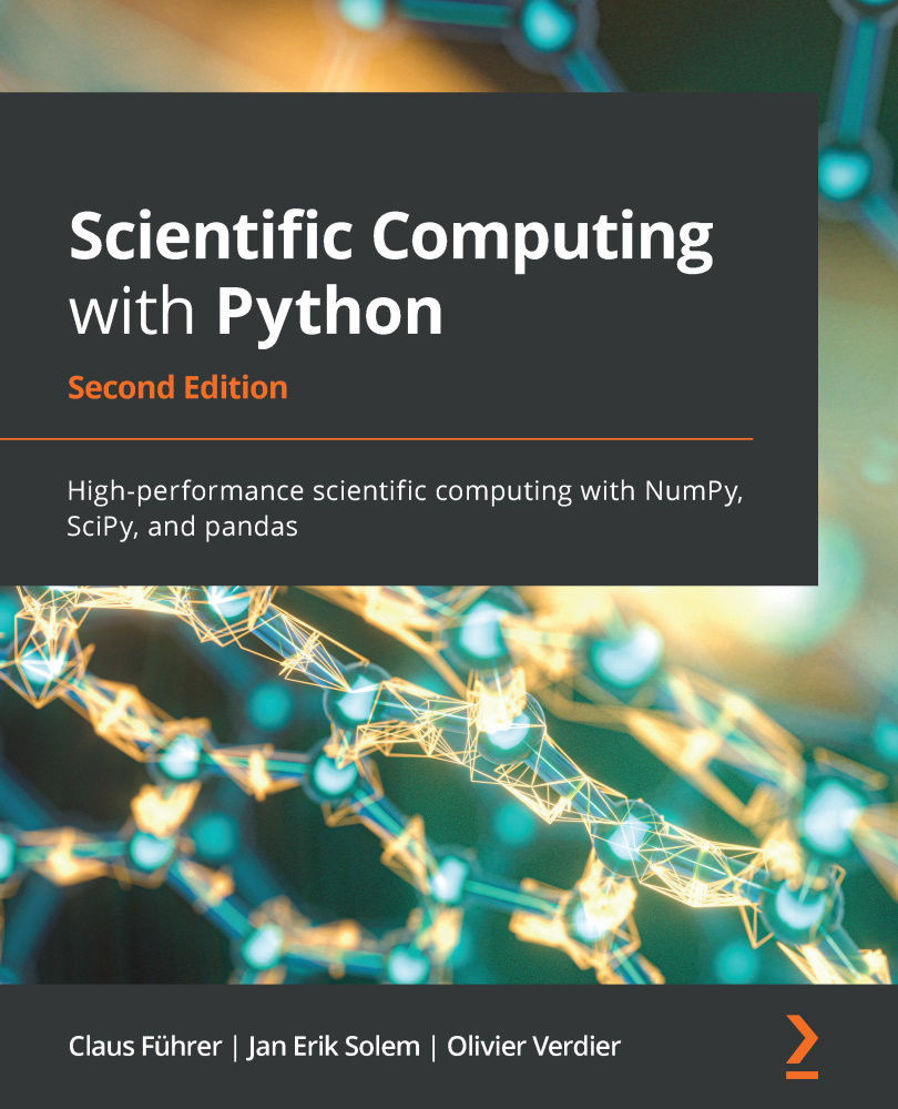
Scientific Computing with Python - Second Edition

Scientific Computing with Python: High-performance scientific computing with NumPy, SciPy, and pandas, Second Edition

By Claus Führer , Jan Erik Solem , Olivier Verdier
€25.99 €17.99
Book Jul 2021 392 pages 2nd Edition
eBook
€25.99 €17.99
Print
€32.99
Subscription
€14.99 Monthly
eBook
€25.99 €17.99
Print
€32.99
Subscription
€14.99 Monthly

What do you get with eBook?

Product feature icon Instant access to your Digital eBook purchase
Product feature icon Download this book in EPUB and PDF formats
Product feature icon Access this title in our online reader with advanced features
Product feature icon DRM FREE - Read whenever, wherever and however you want
Buy Now

Product Details


Publication date : Jul 23, 2021
Length 392 pages
Edition : 2nd Edition
Language : English
ISBN-13 : 9781838822323
Category :
Table of content icon View table of contents Preview book icon Preview Book

Scientific Computing with Python - Second Edition

Variables and Basic Types

In this chapter, we will present the most important and basic types in Python. What is a type? It is a set consisting of data content, its representation, and all possible operations. Later in this book, we will make this definition much more precise when we introduce the concepts of a class in Chapter 8: Classes.

In this chapter, we'll cover the following topics:

  • Variables
  • Numeric types
  • Booleans
  • Strings

2.1 Variables

Variables are references to Python objects. They are created by assignments, for example:

a = 1
diameter = 3.
height = 5.
cylinder = [diameter, height] # reference to a list

Variables take names that consist of any combination of capital and small letters, the underscore _, and digits. A variable name must not start with a digit. Note that variable names are case sensitive. A good naming of variables is an essential part of documenting your work, so we recommend that you use descriptive variable names.

Python has 33 reserved keywords, which cannot be used as variable names (see Table 2.1). Any attempt to use such a keyword as a variable name would raise a syntax error:

Table 2.1: Reserved Python keywords

As opposed to other programming languages, variables require no type declaration in Python. The type is automatically deduced:

x = 3 # integer (int)
y = 'sunny' # string (str)

You can create several variables with a multiple assignment statement:

a = b = c = 1 # a, b and c get the same value 1

Variables can also be altered after their definition:

a = 1 
a = a + 1 # a gets the value 2
a = 3 * a # a gets the value 6

The last two statements can be written by combining the two operations with an assignment directly by using increment operators:

a += 1 # same as a = a + 1 
a *= 3 # same as a = 3 * a

2.2 Numeric types

At some point, you will have to work with numbers, so we start by considering different forms of numeric types in Python. In mathematics, we distinguish between natural numbers (ℕ), integers (ℤ), rational numbers (ℚ), real numbers (ℝ), and complex numbers (ℂ). These are infinite sets of numbers. Operations differ between these sets and may even not be defined. For example, the usual division of two numbers in ℤ might not result in an integer — it is not defined on ℤ.

In Python, like many other computer languages, we have numeric types:

  • The numeric type, int, which is at least theoretically the entire ℤ
  • The numeric type, float, which is a finite subset of ℝ
  • The numeric type, complex, which is a finite subset of ℂ

Finite sets have a smallest and a largest number and there is a minimum spacing between two numbers; see Section 2.2.2Floating-point numbersfor further details.

2.2.1 Integers

The simplest numeric type is the integer type int.

Plain integers

The statement k = 3 assigns the variable k to an integer.

Applying an operation such as +-, or * to integers returns an integer. The division operator, //, returns an integer, while / returns a float:

6 // 2  # 3  an integer value
7 // 2 # 3
7 / 2 # 3.5 a float value

The set of integers in Python is unbounded; there is no largest integer. The limitation here is the computer's memory rather than any fixed value given by the language.

If the division operator (/) in the preceding example returns 3, you have not installed the correct Python version.

2.2.2 Floating-point numbers

If you execute the statement a = 3.0 in Python, you create a floating-point number (Python type: float). These numbers form a finite subset of rational numbers, ℚ.

Alternatively, the constant could have been given in exponent notation as a = 30.0e-1 or simply a = 30.e-1. The symbol e separates the exponent from the mantissa, and the expression reads in mathematical notation as . The name floating-point number refers to the internal representation of these numbers and reflects the floating position of the decimal point when considering numbers over a wide range.

Applying elementary mathematical operations, such as +-*, and /to two floating-point numbers, or to an integer and a floating-point number, returns a floating-point number.

Operations between floating-point numbers rarely return the exact result expected from rational number operations:

0.4 - 0.3 # returns 0.10000000000000003

This fact matters when comparing floating-point numbers:

0.4 - 0.3 == 0.1 # returns False

The reason for this becomes apparent when looking at the internal representation of floating-point numbers; see also Section 15.2.6, Float comparisons.

Floating-point representation

A floating-point number is represented by three quantities: the sign, the mantissa, and the exponent:

with  and .

is called the mantissa,  the basis, and e the exponent, with is called the mantissa length. The condition  makes the representation unique and saves, in the binary case (), one bit.

Two-floating point zeros,  and , exist, both represented by the mantissa .

On a typical Intel processor, . To represent a number in the float type, 64 bits are used, namely, 1 bit for the sign,  bits for the mantissa, and  bits for the exponent . The upper bound  for the exponent is consequently .

With this data, the smallest positive representable number is

, and the largest .

Note that floating-point numbers are not equally spaced in . There is, in particular, a gap at zero (see also [29]). The distance between and the first positive number is , while the distance between the first and the second is smaller by a factor . This effect, caused by the normalization , is visualized in Figure 2.1:

Figure 2.1: The floating-point gap at zero. Here 

This gap is filled equidistantly with subnormal floating-point numbers to which such a result is rounded. Subnormal floating-point numbers have the smallest possible exponent and do not follow the normalization convention, .

Infinite and not a number

There are, in total,  floating-point numbers. Sometimes, a numerical algorithm computes floating-point numbers outside this range.

This generates number overflow or underflow. In NumPy, the special floating-point number inf is assigned to overflow results:

exp(1000.) # inf 
a = inf
3 - a # -inf
3 + a # inf

Working with inf may lead to mathematically undefined results. This is indicated in Python by assigning the result another special floating-point number, nan. This stands for not-a-number, that is, an undefined result of a mathematical operation. To demonstrate this, we continue the previous example:

a + a # inf
a - a # nan
a / a # nan

There are special rules for operations with nan and inf. For instance, nan compared to anything (even to itself) always returns False:

x = nan 
x < 0 # False
x > 0 # False
x == x # False

See Exercise 4 for some surprising consequences of the fact that nan is never equal to itself.

The float inf behaves much more as expected:

0 < inf     # True 
inf <= inf # True
inf == inf # True
-inf < inf # True
inf - inf # nan
exp(-inf) # 0
exp(1 / inf) # 1

One way to check for nan and inf is to use the functions isnan and isinf. Often, you want to react directly when a variable gets the value nan or inf. This can be achieved by using the NumPy command seterr. The following command

seterr(all = 'raise')

would raise a FloatingPointError if a calculation were to return one of those values.

Underflow – Machine epsilon

Underflow occurs when an operation results in a rational number that falls into the gap at zero; see Figure 2.1.

The machine epsilonor rounding unit, is the largest number  such that .

Note that  on most of today's computers. The value that applies on the actual machine you are running your code on is accessible using the following command:

import sys 
sys.float_info.epsilon # 2.220446049250313e-16

The variable sys.float_info contains more information on the internal representation of the float type on your machine.

The function float converts other types to a floating-point number, if possible. This function is especially useful when converting an appropriate string to a number:

a = float('1.356')

Other float types in NumPy

NumPy also provides other float types, known from other programming languages as double-precision and single-precision numbers, namely, float64 and float32:

a = pi            # returns 3.141592653589793 
a1 = float64(a) # returns 3.141592653589793
a2 = float32(a) # returns 3.1415927
a - a1 # returns 0.0
a - a2 # returns -8.7422780126189537e-08

The second last line demonstrates that a and a1 do not differ in accuracy. A difference in accuracy exists between a and its single-precision counterpart, a2.

The NumPy function finfo can be used to display information on these floating-point types:

f32 = finfo(float32) 
f32.precision # 6 (decimal digits)
f64 = finfo(float64)
f64.precision # 15 (decimal digits)
f = finfo(float)
f.precision # 15 (decimal digits)
f64.max # 1.7976931348623157e+308 (largest number)
f32.max # 3.4028235e+38 (largest number)
help(finfo) # Check for more options

2.2.3 Complex numbers

Complex numbers are an extension of the real numbers frequently used in many scientific and engineering fields.

Complex numbers in mathematics

Complex numbers consist of two floating-point numbers, the real part, , of the number, and its imaginary part, . In mathematics, a complex number is written as , where defined by is the imaginary unit. The conjugate complex counterpart of  is .

If the real part  is zero, the number is called an imaginary number.

The j notation

In Python, imaginary numbers are characterized by suffixing a floating-point number with the letter j, for example, z = 5.2j. A complex number is formed by the sum of a real number and an imaginary number, for example, z = 3.5 + 5.2j.

While in mathematics the imaginary part is expressed as a product of a real number b with the imaginary unit , the Python way of expressing an imaginary number is not a product: j is just a suffix to indicate that the number is imaginary.

This is demonstrated by the following small experiment:

b = 5.2 
z = bj # returns a NameError
z = b*j # returns a NameError
z = b*1j # is correct

The method conjugate returns the conjugate of z:

z = 3.2 + 5.2j 
z.conjugate() # returns (3.2-5.2j)

Real and imaginary parts

You may access the real and imaginary parts of a complex number  using the real and imag attributes. Those attributes are read-only; in other words, they cannot be changed:

z = 1j 
z.real # 0.0
z.imag # 1.0
z.imag = 2 # AttributeError: readonly attribute

It is not possible to convert a complex number to a real number:

z = 1 + 0j 
z == 1 # True
float(z) # TypeError

Interestingly, the real and imag attributes as well as the conjugate method work just as well for complex arrays; see also Section 4.3.1, Array properties. We demonstrate this by computing the Nth roots of unity, which are , that is, the  solutions of the equation :

from matplotlib.pyplot import *
N = 10
# the following vector contains the Nth roots of unity:
unity_roots = array([exp(1j*2*pi*k/N) for k in range(N)])
# access all the real or imaginary parts with real or imag:
axes(aspect='equal')
plot(unity_roots.real, unity_roots.imag, 'o')
allclose(unity_roots**N, 1) # True

The resulting figure shows the 10 roots of unity. In Figure 2.2, it is completed by a title and axes labels and shown together with the unit circle. (For more details on how to make plots, see Chapter 6: Plotting.)

Figure 2.2: Roots of unity together with the unit circle

It is, of course, possible to mix the previous methods, as illustrated by the following examples:

z = 3.2+5.2j 
(z + z.conjugate()) / 2. # returns (3.2+0j)
((z + z.conjugate()) / 2.).real # returns 3.2
(z - z.conjugate()) / 2. # returns 5.2j
((z - z.conjugate()) / 2.).imag # returns 5.2
sqrt(z * z.conjugate()) # returns (6.1057350089894991+0j)

2.3 Booleans

Boolean is a data type named after George Boole (1815-1864). A Boolean variable can take only two values, True or False. The main use of this type is in logical expressions. Here are some examples:

a = True 
b = 30 > 45 # b gets the value False

Boolean expressions are often used in conjunction with if statements:

x= 5
if x > 0:
print("positive")
else:
print("nonpositive")

2.3.1 Boolean operators

Boolean operations are performed using the keywords andor, and not:

True and False # False
False or True # True
(30 > 45) or (27 < 30) # True
not True # False
not (3 > 4) # True

The operators follow some precedence rules (see also Section 1.3.5Boolean expressions) which would make the parentheses in the third and in the last line obsolete. Nevertheless, it is a good practice to use them in any case to increase the readability of your code.

Note, the and operator is implicitly chained in the following Boolean expressions:

a < b < c     # same as: a < b and b < c 
a < b <= c # same as: a < b and b <= c (less or equal)
a == b == c # same as: a == b and b == c

2.3.2 Boolean casting

Most Python objects may be converted to Booleans; this is called Boolean casting. The built-in function bool performs that conversion. Note that most objects are cast to True, except 0, the empty tuple, the empty list, the empty string, or the empty array. These are all cast to False.

Table 2.2: Casting rules for Booleans

It is not possible to cast arrays into Booleans unless they contain no or only one element; this is explained further in Section 5.2.1Boolean arrays. The previous table (see Table 2.2: Casting rules for Booleans) contains summarized rules for Boolean casting.

We demonstrate this by means of some usage examples:

bool([]) # False 
bool(0) # False
bool(' ') # True
bool('') # False
bool('hello') # True
bool(1.2) # True
bool(array([1])) # True
bool(array([1,2])) # Exception raised!

Automatic Boolean casting

Using an if statement with a non-Boolean type will cast it to a Boolean. In other words, the following two statements are always equivalent:

if a:
...
if bool(a): # exactly the same as above
...

A typical example is testing whether a list is empty:

# L is a list
if L:
print("list not empty")
else:
print("list is empty")

An empty list, or tuple, will return False.

You can also use a variable in the if statement, for example, an integer:

# n is an integer
if n % 2: # the modulo operator
print("n is odd")
else:
print("n is even")

Note that we used % for the modulo operation, which returns the remainder of an integer division. In this case, it returns 0 or 1 as the remainder after modulo 2.

In this last example, the values 0 or 1 are cast to bool; see also Section 2.3.4, Booleans and integers.

The Boolean operators orand, and not will also implicitly convert some of their arguments to a Boolean.

2.3.3 Return values of and and or

Note that the operators and and or do not necessarily produce Boolean values. This can be explained by the fact that the expression x and y is equivalent to:

def and_as_function(x,y):
if not x:
return x
else:
return y

Correspondingly, the expression x or y is equivalent to:

def or_as_function(x,y):
if x:
return x
else:
return y

Interestingly, this means that when executing the statement True or x, the variable x need not even be defined! The same holds for False and x.

Note that, unlike their counterparts in mathematical logic, these operators are no longer commutative in Python. Indeed, the following expressions are not equivalent:

1 or 'a' # produces 1 
'a' or 1 # produces 'a'

2.3.4 Booleans and integers

In fact, Booleans and integers are the same. The only difference is in the string representations of 0 and 1, which, in the case of Booleans, is False and Truerespectively. This allows constructions such as this:

def print_ispositive(x):
possibilities = ['nonpositive or zero', 'positive']
return f"x is {possibilities[x>0]}"

The last line in this example uses string formatting, which is explained in Section 2.4.3, String formatting.

We note for readers already familiar with the concept of subclasses that the type bool is a subclass of the type int (see Chapter 8: Classes). Indeed, all four inquiries – isinstance(True, bool), isinstance(False, bool), isinstance(True, int), and isinstance(False, int) return the value True (see Section 3.7Checking the type of a variable).

Even rarely used statements such as True+13 are correct.

2.4 Strings

The type string is a type used for text:

name = 'Johan Carlsson'
child = "Åsa is Johan Carlsson's daughter"
book = """Aunt Julia
and the Scriptwriter"""

A string is enclosed either by single or double quotes. If a string contains several lines, it has to be enclosed by three double quotes """ or three single quotes '''.

Strings can be indexed with simple indexes or slices (see  Chapter 3: Container Types, for a comprehensive explanation on slices):

book[-1] # returns 'r' 
book[-12:] # returns 'Scriptwriter'

Strings are immutable; that is, items cannot be altered. They share this property with tuples. The command book[1] = 'a' returns:

TypeError: 'str' object does not support item assignment

2.4.1 Escape sequences and raw strings

The string '\n' is used to insert a line break and '\t' inserts a horizontal tabulator (TAB) into the string to align several lines:

print('Temperature\t20\tC\nPressure\t5\tPa')

These strings are examples of escape sequences. Escape sequences always start with a backslash, \. A multiline string automatically includes escape sequences:

a=""" 
A multi-line
example"""
a # returns '\nA multi-line \nexample'

A special escape sequence is "\\", which represents the backslash symbol in text:

latexfontsize="\\tiny"
print(latexfontsize) # prints \tiny

The same can be achieved by using a raw string instead:

latexfs=r"\tiny" # returns "\tiny"
latexfontsize == latexfs # returns True

Note that in raw strings, the backslash remains in the string and is used to escape some special characters:

print(r"\"") # returns \"
print(r"\\") # returns \
print(r"\") # returns an error (why?)

A raw string is a convenient tool to construct strings in a readable manner. The result is the same:

r"\"" == '\\"'
r"She: \"I am my dad's girl\"" == 'She: \\"I am my dad\'s girl\\"'

2.4.2 Operations on strings and string methods

The addition of several strings results in their concatenation:

last_name = 'Carlsson'
first_name = 'Johanna'
full_name = first_name + ' ' + last_name
# returns 'Johanna Carlsson'

Consequently, multiplication by an integer is repeated addition:

game = 2 * 'Yo' # returns 'YoYo'

Multiplication by floating-point or complex numbers is undefined and results in a TypeError.

When strings are compared, lexicographical order applies and the uppercase form precedes the lowercase form of the same letter:

'Anna' > 'Arvi' # returns false 
'ANNA' < 'anna' # returns true
'10B' < '11A' # returns true

Among the variety of string methods, we will mention here only the most important ones:

  • Splitting a string: This method generates a list from a string by using a single or multiple blanks as separators. Alternatively, an argument can be given by specifying a particular substring as a separator:
text = 'quod erat demonstrandum'
text.split() # returns ['quod', 'erat', 'demonstrandum']
table = 'Johan;Carlsson;19890327'
table.split(';') # returns ['Johan','Carlsson','19890327']
king = 'CarlXVIGustaf'
king.split('XVI') # returns ['Carl','Gustaf']
  • Joining a list to a string: This is the reverse operation of splitting:
sep = ';'
sep.join(['Johan','Carlsson','19890327'])
# returns 'Johan;Carlsson;19890327'
  • Searching in a string: This method returns the first index in the string, where a given search substring starts:
birthday = '20101210'
birthday.find('10') # returns 2

If the search string is not found, the return value of the method is -1.

  • String formatting: This method inserts values of variables or results of expressions into a string. It is so important that we devote the following subsection to it. 

2.4.3 String formatting

String formatting is the process of inserting values into a given string and determining the way in which they are displayed. This can be done in various ways. We first describe the related string method, format, and the more modern alternative, the so-called f-string

Here is an example regarding the use of the format method:

course_code = "NUMA01"
print("Course code: {}".format(course_code)) # Course code: NUMA01

And here is an example of the variant by using an f-string:

course_code = "NUMA01"
print(f"Course code: {course_code}")
# Course code: NUMA01

The function format is a string method; it scans the string for the occurrence of placeholders, which are enclosed by curly brackets. These placeholders are replaced in a way specified by the argument of the format method. How they are replaced depends on the format specification defined in each {} pair. Format specifications are indicated by a colon, ":", as their prefix.

The format method offers a range of possibilities to customize the formatting of objects depending on their types. Of particular use in scientific computing are the formatting specifiers for the float type. You may choose either the standard fixed-point notation with {:f} or the exponential notation with {:e}:

quantity = 33.45
print("{:f}".format(quantity)) # 33.450000
print("{:1.1f}".format(quantity)) # 33.5
print("{:.2e}".format(quantity)) # 3.35e+01

Similarly, format specifiers can be used also in f-strings:

quantity = 33.45
print(f"{quantity:1.1f}") # 33.5

The format specifiers allow specifying the rounding precision (digits following the decimal point in the representation). Also, the total number of symbols, including leading blanks, to represent the number can be set.

In this example, the name of the object that gets its value inserted is given as an argument to the format method. The first {} pair is replaced by the first argument, and the following pairs by the subsequent arguments. Alternatively, it may also be convenient to use the key-value syntax:

print("{name} {value:.1f}".format(name="quantity",value=quantity))
# prints "quantity 33.5"

Here, two values are processed – a string name without a format specifier, and a float value that is printed in fixed-point notation with one digit after the decimal point. (Refer to the complete reference documentation for more details on string formatting.)

Braces in the string

Sometimes, a string might contain a pair of curly braces, which should not be considered as placeholders for a format method. In that case, double braces are used:

r"we {} in LaTeX \begin{{equation}}".format('like')

This returns the following string: 'we like in LaTeX \\begin{equation}'.

2.5 Summary

In this chapter, you met the basic data types in Python and saw the corresponding syntax elements. We will work mostly with numeric types such as integers, floats, and complex.

Booleans are needed for setting conditions, and by using strings, we often communicate results and messages.

2.6 Exercises

Ex. 1: Check whether  is a zero of the function:

Ex. 2: According to de Moivre's formula, the following holds:

Choose numbers n and x and verify that formula in Python.

Ex. 3: Complex numbers. Verify Euler's formula in the same way:

Ex. 4: Suppose we are trying to check the convergence of a diverging sequence (here, the sequence is defined by the recursive relation  and ):

u = 1.0 # you have to use a float here!
uold = 10.
for iteration in range(2000):
if not abs(u-uold) > 1.e-8:
print('Convergence')
break # sequence has converged
uold = u
u = 2*u
else:
print('No convergence')
  1. Since the sequence does not converge, the code should print the
     No convergence message. Execute it to see what happens.
  1. What happens if you replace the line
      if not abs(u-uold) > 1.e-8:

with

      if abs(u-uold) < 1.e-8:

It should give exactly the same result, shouldn't it? Run the code again to see what happens.

  1. What happens if you replace u=1.0 with u=1 (without a decimal point)? Run the code to check your predictions.
  2. Explain the unexpected behavior of this code.

Ex. 5: An implication C = (A ⇒ B) is a Boolean expression that is defined as

  • C is True if A is Falseor A and B are both True
  • C is False otherwise

Write a Python function implication(A, B).

Ex. 6: This exercise is to train Boolean operations. Two binary digits (bits) are added by using a logical device called a half adder. It produces a carry bit (the digit of the next higher value) and the sum as defined by the following table, and half adder circuit:

p
q
sum
carry
1
1
0
1
1
0
1
0
0
1
1
0
0
0
0
0


Definition of the half adder operation:

Figure 2.3: A half adder circuit

A full adder consists of two half adders and sums two bits and an additional carry bit on the input (see also the following figure):

Figure 2.4: A full adder circuit

Write a function that implements a half adder and another that implements a full adder. Test these functions.

Left arrow icon Right arrow icon
Download code icon Download Code

Key benefits

  • Learn the first steps within Python to highly specialized concepts
  • Explore examples and code snippets taken from typical programming situations within scientific computing.
  • Delve into essential computer science concepts like iterating, object-oriented programming, testing, and MPI presented in strong connection to applications within scientific computing.

Description

Python has tremendous potential within the scientific computing domain. This updated edition of Scientific Computing with Python features new chapters on graphical user interfaces, efficient data processing, and parallel computing to help you perform mathematical and scientific computing efficiently using Python. This book will help you to explore new Python syntax features and create different models using scientific computing principles. The book presents Python alongside mathematical applications and demonstrates how to apply Python concepts in computing with the help of examples involving Python 3.8. You'll use pandas for basic data analysis to understand the modern needs of scientific computing, and cover data module improvements and built-in features. You'll also explore numerical computation modules such as NumPy and SciPy, which enable fast access to highly efficient numerical algorithms. By learning to use the plotting module Matplotlib, you will be able to represent your computational results in talks and publications. A special chapter is devoted to SymPy, a tool for bridging symbolic and numerical computations. By the end of this Python book, you'll have gained a solid understanding of task automation and how to implement and test mathematical algorithms within the realm of scientific computing.

What you will learn

Understand the building blocks of computational mathematics, linear algebra, and related Python objects Use Matplotlib to create high-quality figures and graphics to draw and visualize results Apply object-oriented programming (OOP) to scientific computing in Python Discover how to use pandas to enter the world of data processing Handle exceptions for writing reliable and usable code Cover manual and automatic aspects of testing for scientific programming Get to grips with parallel computing to increase computation speed

What do you get with eBook?

Product feature icon Instant access to your Digital eBook purchase
Product feature icon Download this book in EPUB and PDF formats
Product feature icon Access this title in our online reader with advanced features
Product feature icon DRM FREE - Read whenever, wherever and however you want
Buy Now

Product Details


Publication date : Jul 23, 2021
Length 392 pages
Edition : 2nd Edition
Language : English
ISBN-13 : 9781838822323
Category :

Table of Contents

23 Chapters
Preface Chevron down icon Chevron up icon
Getting Started Chevron down icon Chevron up icon
Variables and Basic Types Chevron down icon Chevron up icon
Container Types Chevron down icon Chevron up icon
Linear Algebra - Arrays Chevron down icon Chevron up icon
Advanced Array Concepts Chevron down icon Chevron up icon
Plotting Chevron down icon Chevron up icon
Functions Chevron down icon Chevron up icon
Classes Chevron down icon Chevron up icon
Iterating Chevron down icon Chevron up icon
Series and Dataframes - Working with Pandas Chevron down icon Chevron up icon
Communication by a Graphical User Interface Chevron down icon Chevron up icon
Error and Exception Handling Chevron down icon Chevron up icon
Namespaces, Scopes, and Modules Chevron down icon Chevron up icon
Input and Output Chevron down icon Chevron up icon
Testing Chevron down icon Chevron up icon
Symbolic Computations - SymPy Chevron down icon Chevron up icon
Interacting with the Operating System Chevron down icon Chevron up icon
Python for Parallel Computing Chevron down icon Chevron up icon
Comprehensive Examples Chevron down icon Chevron up icon
About Packt Chevron down icon Chevron up icon
Other Books You May Enjoy Chevron down icon Chevron up icon
References Chevron down icon Chevron up icon

Customer reviews

Filter icon Filter
Top Reviews
Rating distribution
Empty star icon Empty star icon Empty star icon Empty star icon Empty star icon 0
(0 Ratings)
5 star 0%
4 star 0%
3 star 0%
2 star 0%
1 star 0%

Filter reviews by


No reviews found
Get free access to Packt library with over 7500+ books and video courses for 7 days!
Start Free Trial

FAQs

How do I buy and download an eBook? Chevron down icon Chevron up icon

Where there is an eBook version of a title available, you can buy it from the book details for that title. Add either the standalone eBook or the eBook and print book bundle to your shopping cart. Your eBook will show in your cart as a product on its own. After completing checkout and payment in the normal way, you will receive your receipt on the screen containing a link to a personalised PDF download file. This link will remain active for 30 days. You can download backup copies of the file by logging in to your account at any time.

If you already have Adobe reader installed, then clicking on the link will download and open the PDF file directly. If you don't, then save the PDF file on your machine and download the Reader to view it.

Please Note: Packt eBooks are non-returnable and non-refundable.

Packt eBook and Licensing When you buy an eBook from Packt Publishing, completing your purchase means you accept the terms of our licence agreement. Please read the full text of the agreement. In it we have tried to balance the need for the ebook to be usable for you the reader with our needs to protect the rights of us as Publishers and of our authors. In summary, the agreement says:

  • You may make copies of your eBook for your own use onto any machine
  • You may not pass copies of the eBook on to anyone else
How can I make a purchase on your website? Chevron down icon Chevron up icon

If you want to purchase a video course, eBook or Bundle (Print+eBook) please follow below steps:

  1. Register on our website using your email address and the password.
  2. Search for the title by name or ISBN using the search option.
  3. Select the title you want to purchase.
  4. Choose the format you wish to purchase the title in; if you order the Print Book, you get a free eBook copy of the same title. 
  5. Proceed with the checkout process (payment to be made using Credit Card, Debit Cart, or PayPal)
Where can I access support around an eBook? Chevron down icon Chevron up icon
  • If you experience a problem with using or installing Adobe Reader, the contact Adobe directly.
  • To view the errata for the book, see www.packtpub.com/support and view the pages for the title you have.
  • To view your account details or to download a new copy of the book go to www.packtpub.com/account
  • To contact us directly if a problem is not resolved, use www.packtpub.com/contact-us
What eBook formats do Packt support? Chevron down icon Chevron up icon

Our eBooks are currently available in a variety of formats such as PDF and ePubs. In the future, this may well change with trends and development in technology, but please note that our PDFs are not Adobe eBook Reader format, which has greater restrictions on security.

You will need to use Adobe Reader v9 or later in order to read Packt's PDF eBooks.

What are the benefits of eBooks? Chevron down icon Chevron up icon
  • You can get the information you need immediately
  • You can easily take them with you on a laptop
  • You can download them an unlimited number of times
  • You can print them out
  • They are copy-paste enabled
  • They are searchable
  • There is no password protection
  • They are lower price than print
  • They save resources and space
What is an eBook? Chevron down icon Chevron up icon

Packt eBooks are a complete electronic version of the print edition, available in PDF and ePub formats. Every piece of content down to the page numbering is the same. Because we save the costs of printing and shipping the book to you, we are able to offer eBooks at a lower cost than print editions.

When you have purchased an eBook, simply login to your account and click on the link in Your Download Area. We recommend you saving the file to your hard drive before opening it.

For optimal viewing of our eBooks, we recommend you download and install the free Adobe Reader version 9.