Working in interactive mode

Matplotlib can be used in an interactive or non-interactive modes. In the interactive mode, the graph display gets updated after each statement. In the non-interactive mode, the graph does not get displayed until explicitly asked to do so.

Getting ready

You need working installations of Python, NumPy, and Matplotlib packages.

Using the following commands, interactive mode can be set on or off, and also checked for current mode at any point in time:

• matplotlib.pyplot.ion() to set the interactive mode ON
• matplotlib.pyplot.ioff() to switch OFF the interactive mode
• matplotlib.is_interactive() to check whether the interactive mode is ON (True) or OFF (False)

How to do it...

Let's see how simple it is to work in interactive mode:

1. Set the screen output as the backend:

%matplotlib inline

2. Import the matplotlib and pyplot libraries. It is common practice in Python to import libraries with crisp synonyms. Note plt is the synonym for the matplotlib.pyplot package:

import matplotlib as mpl
import matplotlib.pyplot as plt

3. Set the interactive mode to ON:

plt.ion()

4. Check the status of interactive mode:

mpl.is_interactive()

5. You should get the output as True.
6. Plot a line graph:

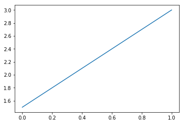
plt.plot([1.5, 3.0])

You should see the following graph as the output:

7. Now add the axis labels and a title to the graph with the help of the following code:

# Add labels and title
plt.title("Interactive Plot") #Prints the title on top of graph
plt.xlabel("X-axis")         # Prints X axis label as "X-axis"
plt.ylabel("Y-axis")         # Prints Y axis label as "Y-axis"

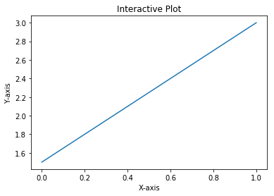
After executing the preceding three statements, your graph should look as follows:

How it works...

So, this is how the explanation goes:

• plt.plot([1.5, 3.0]) plots a line graph connecting two points (0, 1.5) and (1.0, 3.0).
• The plot command expects two arguments (Python list, NumPy array or pandas DataFrame) for the x and y axis respectively.
• If only one argument is passed, it takes it as y axis co-ordinates and for x axis co-ordinates it takes the length of the argument provided.
• In this example, we are passing only one list of two points, which will be taken as y axis coordinates.
• For the x axis, it takes the default values in the range of 0 to 1, since the length of the list [1.5, 3.0] is 2.
• If we had three coordinates in the list for y, then for x, it would take the range of 0 to 2.
• You should see the graph like the one shown in step 6.
• plt.title("Interactive Plot"), prints the title on top of the graph as Interactive Plot.
• plt.xlabel("X-axis"), prints the x axis label as X-axis.
• plt.ylabel("Y-axis"), prints the y axis label as Y-axis.
• After executing preceding three statements, you should see the graph as shown in step 7.

If you are using Python shell, after executing each of the code statements, you should see the graph getting updated with title first, then the x axis label, and finally the y axis label.

If you are using Jupyter Notebook, you can see the output only after all the statements in a given cell are executed, so you have to put each of these three statements in separate cells and execute one after the other, to see the graph getting updated after each code statement.

In older versions of Matplotlib or certain backends (such as macosx), the graph may not be updated immediately. In such cases, you need to call plt.draw() explicitly at the end, so that the graph gets displayed.

There's more...

You can add one more line graph to the same plot and go on until you complete your interactive session:

1. Plot a line graph:

plt.plot([1.5, 3.0])

2. Add labels and title:

plt.title("Interactive Plot")
plt.xlabel("X-axis")
plt.ylabel("Y-axis")

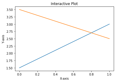
3. Add one more line graph:

plt.plot([3.5, 2.5])

The following graph is the output obtained after executing the code:

Hence, we have now worked in interactive mode.