Search icon CANCEL
Subscription
0
Cart icon
Your Cart (0 item)
Close icon
You have no products in your basket yet
Save more on your purchases! discount-offer-chevron-icon
Savings automatically calculated. No voucher code required.
Arrow left icon
Explore Products
Best Sellers
New Releases
Books
Videos
Audiobooks
Learning Hub
Newsletter Hub
Free Learning
Arrow right icon
timer SALE ENDS IN
0 Days
:
00 Hours
:
00 Minutes
:
00 Seconds
Time Series Analysis with Python Cookbook

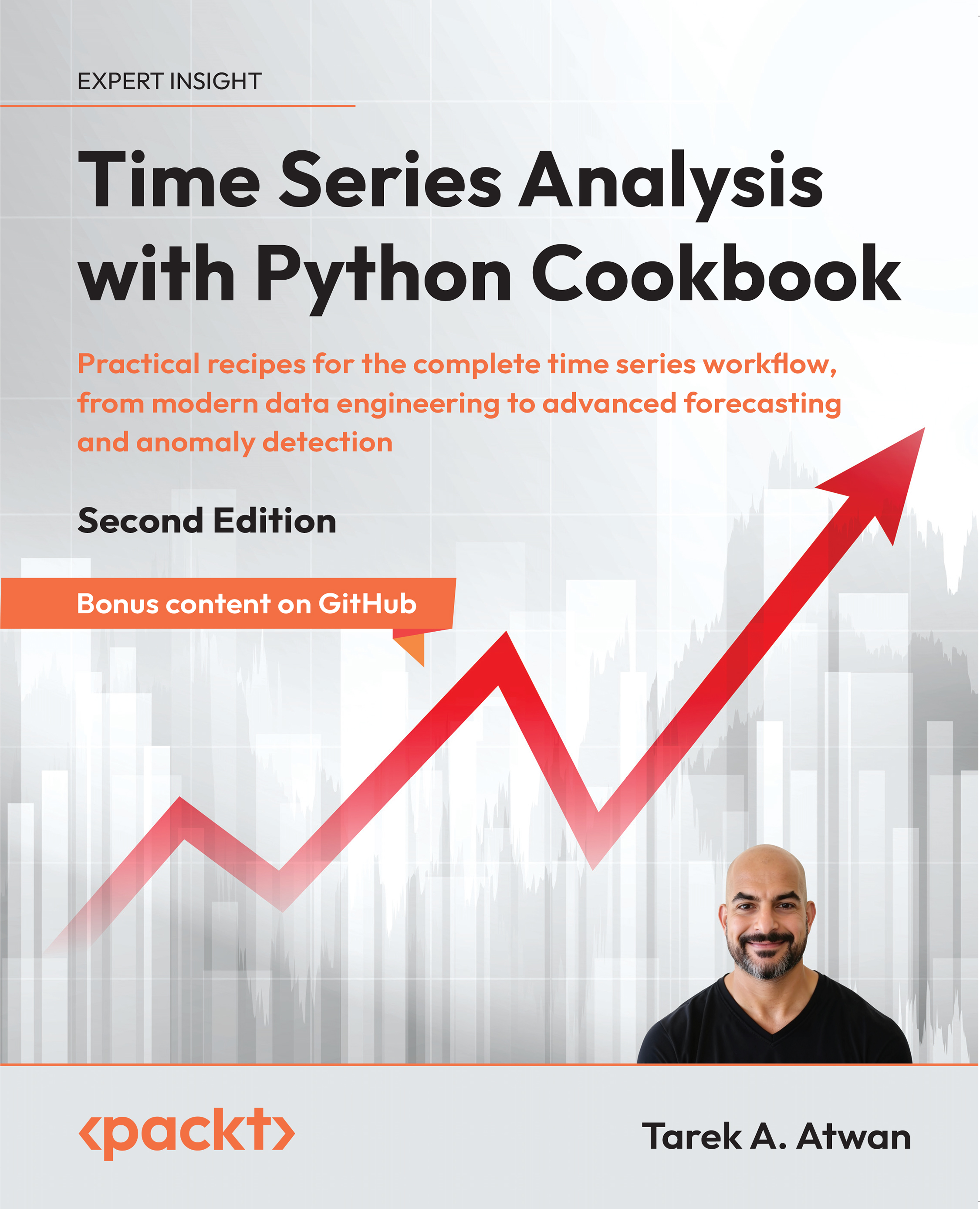
Time Series Analysis with Python Cookbook: Practical recipes for the complete time series workflow, from modern data engineering to advanced forecasting and anomaly detection , Second Edition

Arrow left icon
Profile Icon Tarek A. Atwan
Arrow right icon
Early Access Early Access Publishing in Jan 2026
€8.98 €35.99
eBook Jan 2026 812 pages 2nd Edition
eBook
€8.98 €35.99
Paperback
€44.99
Subscription
Free Trial
Renews at €18.99p/m
Arrow left icon
Profile Icon Tarek A. Atwan
Arrow right icon
Early Access Early Access Publishing in Jan 2026
€8.98 €35.99
eBook Jan 2026 812 pages 2nd Edition
eBook
€8.98 €35.99
Paperback
€44.99
Subscription
Free Trial
Renews at €18.99p/m
eBook
€8.98 €35.99
Paperback
€44.99
Subscription
Free Trial
Renews at €18.99p/m

What do you get with eBook?

Product feature icon Instant access to your Digital eBook purchase
Product feature icon Download this book in EPUB and PDF formats
Product feature icon Access this title in our online reader with advanced features
Product feature icon DRM FREE - Read whenever, wherever and however you want
Modal Close icon
Payment Processing...
tick Completed

Billing Address

Table of content icon View table of contents Preview book icon Preview Book

Time Series Analysis with Python Cookbook

Reading Time Series Data from Files

Time series analysis often begins with data preparation, a crucial and time-consuming stage. To effectively analyze time series, you first need to access the data, often stored in various file formats or database systems.

Time series data is complex and can appear in various shapes and formats. For instance, it may come as regular timestamped records, such as hourly temperature readings, or irregular events, such as transaction logs with varying time intervals. Data might also include multiple time series combined into a single dataset, such as sales and inventory levels for several stores.

In this chapter, we will use pandas, a popular Python library with a rich set of I/O tools, data wrangling, and date/time handling capabilities that streamline the process of working with time series data. You will explore several of the reader functions available in pandas to ingest data from different file types, including comma-separated values (CSV), Excel, and Parquet. Additionally, you will explore ingesting data from files stored locally or remotely on the cloud, such as an Amazon S3 bucket.

The pandas library provides two fundamental data structures for working with time series data: Series and DataFrame. A DataFrame is a distinct data structure for working with tabular data (think rows and columns in a spreadsheet). The main difference between the two data structures is that a Series is one-dimensional (single column), while a DataFrame is two-dimensional (multiple columns). The relationship between the two is that you get a Series when you slice out a column from a DataFrame. You can think of a DataFrame as a side-by-side concatenation of two or more Series objects.

A particular feature of the Series and DataFrames data structures is that they both have a labeled axis called an index. A specific type of index that you will often see with time series data is DatetimeIndex, which you will explore further in this chapter. Generally, the index makes slicing and dicing operations very intuitive. For example, to make a DataFrame ready for time series analysis, you will learn how to create DataFrames with an index of the DatetimeIndex type.

The recipes in this chapter will guide you through key techniques to load time series data into pandas DataFrames:

  • Reading data from CSV and other delimited files
  • Reading data from an Excel file
  • Reading data from URLs
  • Reading data from Parquet files

There’s an exciting GitHub-only bonus—Chapter 0: Getting Started with Time Series Analysis—available here: https://github.com/PacktPublishing/Time-Series-Analysis-with-Python-Cookbook-Second-Edition

Don’t miss the GitHub-exclusive recipe— Chapter 1-1: Working with large data files—available here: https://github.com/PacktPublishing/Time-Series-Analysis-with-Python-Cookbook-Second-Edition

Why DateTimeIndex?

A pandas DataFrame with an index of the DatetimeIndex type unlocks a large set of features and useful functions needed when working with time series data. You can think of it as adding a layer of intelligence or awareness to pandas to treat the DataFrame as a time series DataFrame.

Free Benefits with Your Book

Your purchase includes a free PDF copy of this book along with other exclusive benefits. Check the Free Benefits with Your Book section in the Preface to unlock them instantly and maximize your learning experience.

Technical requirements

In this chapter and forward, you will extensively use pandas 2.3.3 (released September 29, 2025).

Throughout our journey, you will be installing additional Python libraries to use in conjunction with pandas. You can download the Jupyter notebooks from the GitHub repository (https://github.com/PacktPublishing/Time-Series-Analysis-with-Python-Cookbook-Second-Edition/blob/main/code/Ch1/Chapter_1.ipynb) to follow along.

You can download the datasets used in this chapter from the GitHub repository using this link: https://github.com/PacktPublishing/Time-Series-Analysis-with-Python-Cookbook-Second-Edition/tree/main/datasets/Ch1.

Reading data from CSV and other delimited files

In this recipe, you will use the pandas.read_csv() function, which offers a large set of parameters that you will explore to ensure that the data is properly read into a time series DataFrame. In addition, you will learn how to specify an index column, parse the index to be of the DatetimeIndex type, and parse string columns that contain dates into datetime objects. A properly parsed DatetimeIndex allows for efficient slicing, resampling, and analysis of time-based data.

CSV files store data in plain text, and when using Python to read data from a CSV file (for example, using the csv Python module), it will be treated as a string (text) by default. In pandas, when using the read_csv() method, it will try to infer the appropriate data types (dtype), and, in most cases, it does a great job at that. However, there are situations where you will need to explicitly indicate which columns to cast to a specific data type. For example, you will specify which column(s) to parse as dates using the parse_dates parameter in this recipe.

Getting ready

You will read a CSV file containing hypothetical box office numbers for a movie. The file is provided in the GitHub repository for this book. The data file is in datasets/Ch1/movieboxoffice.csv.

How to do it…

You will ingest our CSV file using pandas and leverage some of the available parameters in read_csv:

  1. Import pandas and Path from pathlib to handle file paths :
    import pandas as pd
    from pathlib import Path
    
  2. Create a Path object for the file location:
    filepath = Path('../../datasets/Ch1/movieboxoffice.csv')
    

Using Path objects is a best practice for cross-platform compatibility, ensuring that your code runs smoothly on Windows, macOS, or Linux.

  1. Read the CSV file into a DataFrame using the read_csv function and pass the filepath with additional parameters.

The first column in the CSV file contains movie release dates, and it needs to be set as an index of the DatetimeIndex type (using index_col=0 and parse_dates=['Date']). Specify which columns you want to include by providing a list of column names to usecols. The default behavior is that the first row includes the header (header=0):

ts = pd.read_csv(filepath,
                 header=0,
                 parse_dates=['Date'],
                 index_col=0,
                 usecols=['Date',
                          'DOW',
                          'Daily',
                          'Forecast',
                          'Percent Diff'])
ts.head(5)

This will output the following first five rows:

                DOW         Daily      Forecast Percent Diff
Date                                                       
2021-04-26    Friday  $125,789.89   $235,036.46       -46.48%
2021-04-27  Saturday   $99,374.01   $197,622.55       -49.72%
2021-04-28    Sunday   $82,203.16   $116,991.26       -29.74%
2021-04-29    Monday   $33,530.26    $66,652.65       -49.69%
2021-04-30   Tuesday   $30,105.24    $34,828.19       -13.56%
  1. Print a summary of the DataFrame to check the index and column data types. Alternatively, you can use raw string r'[^\d.-]' to avoid double backslashes.:
    ts.info()
    >> <class 'pandas.core.frame.DataFrame'>
    DatetimeIndex: 128 entries, 2021-04-26 to 2021-08-31
    Data columns (total 4 columns):
     #   Column        Non-Null Count  Dtype
    ---  ------        --------------  -----
     0   DOW           128 non-null    object
     1   Daily         128 non-null    object
     2   Forecast      128 non-null    object
     3   Percent Diff  128 non-null    object
    dtypes: object(4)
    memory usage: 5.0+ KB
    

Notice that the Date column is now an index (not a column) of the DatetimeIndex type. Additionally, the Daily, Forecast, and Percent Diff columns have the wrong dtype inference. You would expect them to be of the float type. The issue is due to the source CSV file containing non-numeric characters, such as dollar signs ($), percent signs (%), and thousand separators (,). The presence of these non-numeric characters can lead to incorrect dtype inference. A column with the dtype object indicates either a string column or a column with mixed dtypes (not homogeneous).

  1. Remove non-numeric characters such as the dollar sign ($), percent sign (%), and thousand separators (,) using str.replace() with a regular expression. The regular expression will remove all non-numeric characters but exclude the decimal points (.) and negative sign (-). Removing these characters does not convert the dtype, so you will need to cast the columns to the float dtype using the astype(float) method:
    clean = lambda x: x.str.replace('[^\\d.-]', '', regex=True) 
    c_df = ts[['Daily', 'Forecast', 'Percent Diff']].apply(clean)
    ts[['Daily', 'Forecast', 'Percent Diff']] = c_df.astype(float)
    

The [^\d.-] regex (written as '[^\\d.-]' in Python strings) breaks down as follows:

  • ^: Matches characters not in the set that follows
  • \d: Matches any digit (0–9)
  • .: Matches the decimal point
  • -: Matches negative signs for negative numbers

Note that we need to use double backslashes in the Python string ('\\d') to escape the backslash character and properly represent a single backslash in the regex pattern ('\d'). Without proper escaping, Python would interpret \d as an invalid string escape sequence before it’s processed as a regex.

Print a summary of the updated DataFrame:

ts.info()
>> <class 'pandas.core.frame.DataFrame'>
<class 'pandas.core.frame.DataFrame'>
DatetimeIndex: 128 entries, 2021-04-26 to 2021-08-31
Data columns (total 4 columns):
 #   Column        Non-Null Count  Dtype
---  ------        --------------  -----
 0   DOW           128 non-null    object
 1   Daily         128 non-null    float64
 2   Forecast      128 non-null    float64
 3   Percent Diff  128 non-null    float64
dtypes: float64(3), object(1)
memory usage: 5.0+ KB

Now, the Daily, Forecast, and Percent Diff columns are of the float64 type, making them suitable for numerical operations and analysis. DatetimeIndex allows for efficient slicing and resampling of time-based data, while the cleaned numeric columns are ready for further calculations

How it works…

Using pandas for data transformation is fast since it loads the data into memory. For example, the read_csv() method reads and loads the entire data into a DataFrame in memory. When requesting a DataFrame summary with the info() method, the output will display memory usage for the entire DataFrame in addition to column data types and index information. To get the exact memory usage for each column, including the index, you can use the memory_usage() method.

The memory_usage() method returns the memory consumption in bytes for each column and the index. The total memory usage (in bytes) matches the memory usage reported in the DataFrame summary:

ts.memory_usage().sum()
>> 5120

So far, you have used a few of the available parameters when reading a CSV file using read_csv(). The more familiar you become with the different options available in any pandas reader functions, the more upfront preprocessing you can do during data ingestion (reading). Keep in mind, though, that while performing transformations during data ingestion reduces subsequent processing, it may slightly increase load time for very large datasets.

You used the built-in parse_dates argument, which accepts a list of columns specified by name or position. The combination of index_col=0 and parse_dates=[0] produced a DataFrame with an index of the DatetimeIndex type. When working with the parse_dates parameter, it’s good practice to verify that your dates were correctly parsed by checking the DataFrame’s index type using type(ts.index). If it returns pandas.core.indexes.datetimes.DatetimeIndex, your parsing was successful. If not, you may need to use date_format or to_datetime(), as described in the There’s more section.

Let’s inspect the parameters used in this recipe as defined in the official pandas.read_csv() documentation (https://pandas.pydata.org/pandas-docs/stable/reference/api/pandas.read_csv.html):

  • filepath_or_buffer: This is the first positional argument and the only required field needed (at a minimum) to read a CSV file. Here, you passed the Python path object named filepath. This can also be a string that represents a valid file path, such as '../../datasets/Ch1/movieboxoffice.csv' or a URL that points to a remote file location, such as an Amazon S3 bucket (we will examine this later in the Reading data from URLs recipe in this chapter).
  • sep: This takes a string to specify which delimiter to use. The default is a comma delimiter (,) which assumes a CSV file. If the file is separated by another delimiter, such as a pipe (|) or semicolon (;), then the argument can be updated, such as sep="|" or sep=";".
  • delimiter: This is an alias to sep, which can be used as well as a parameter name.
  • header: In this case, you specified that the first row (0) value contains the header information. The default value is infer, which usually works as-is in most cases. If the CSV does not contain a header, then you specify header=None. If the CSV has a header but you prefer to supply custom column names, then you need to specify header=0 and overwrite it by providing a list of new column names to the names argument.
  • parse_dates: In the recipe, you provided a list of column positions using [0], which specified that only the first column (by position) should be parsed. The parse_dates argument can take a list of column names, such as ["Date"], or a list of column positions, such as [0, 3], indicating the first and the fourth columns. If you only intend to parse the index column(s) specified in the index_col parameter, you only need to pass True (Boolean).
  • index_col: You specified that the first column by position (index_col=0) will be used as the DataFrame index. Alternatively, you could provide the column name as a string (index_col='Date'). The parameter also takes in a list of integers (positional indices) or strings (column names), which would create a MultiIndex object.
  • usecols: The default value is None, which includes all the columns in the dataset. Limiting the number of columns to only those that are required results in faster parsing and overall lower memory usage, since you only bring in what is needed. The usecols argument can take a list of column names, such as ['Date', 'DOW', 'Daily', 'Percent Diff', 'Forecast'] or a list of positional indices, such as [0, 1, 3, 7, 6], which would produce the same result.

Recall that you specified which columns to include by passing a list of column names to the usecols parameter. These names are based on the file header (the first row of the CSV file). Generally, the combination of usecols and header is especially useful when working with large files.

If you provide custom header names, you cannot reference the original names in the usecols parameter; this will produce the following error: ValueError: Usecols do not match columns. Instead, you can use column positions or rename the columns in two steps. The following are two approaches to handle this:

col_names = ['Date', 'Day Name', 'Daily BO', 'Forecast BO']
df = pd.read_csv(filepath,
                 parse_dates=[0],
                 index_col=0,
                 header=0,
                 names=col_names,
                 usecols=[0, 1, 3, 6])

By using column positions in usecols, you bypass the need for matching column names, which allows you to apply custom headers without encountering errors

Alternatively, you can accomplish this in two steps using a Python dictionary:

col_names = {
    'Date': 'Date',
    'DOW': 'Day Name',
    'Daily': 'Daily BO',
    'Forecast': 'Forecast BO'
}
df = pd.read_csv(filepath,
                 parse_dates=[0],
                 index_col=0,
                 usecols=col_names.keys())
df.rename(columns=col_names, inplace=True)

Using a dictionary to map original column names to new ones allows flexibility and clarity, especially when dealing with large datasets or when you need to maintain a reference to original column names.

There’s more…

There are situations where parse_dates may not work (it just cannot parse the date). In such cases, the column(s) will be returned unchanged, and no error will be thrown. This is where the date_format parameter can be helpful.

The following code shows how date_format can be used:

ts = pd.read_csv(filepath,
                 parse_dates=[0],
                 index_col=0,
                 date_format="%d-%b-%Y",
                 usecols=[0,1,3, 7, 6])
ts.head()

The preceding code will print out the first five rows of the ts DataFrame, displaying a correctly parsed Date index.

Let’s break it down. In the preceding code, since the date is stored as a string in the form 26-Apr-2021, you passed "%d-%b-%Y" to reflect that:

  • %d represents the day of the month, such as 01 or 02
  • %b represents the abbreviated month name, such as Apr or May
  • %Y represents the year as a four-digit number, such as 2020 or 2021

Other common string codes include the following:

  • %y represents a two-digit year, such as 19 or 20
  • %B represents the month’s full name, such as January or February
  • %m represents the month as a two-digit number, such as 01 or 02

For more information on Python’s string formats for representing dates, visit https://strftime.org.

When dealing with more complex date formats, an alternative option is to use the to_datetime() function. The to_datetime() function is used to convert a string, integer, or float into a datetime object.

Initially, you will read the CSV data as is, then apply the to_datetime() function to parse the specific column(s) as desired. This is demonstrated in the following code:

ts = pd.read_csv(filepath,
                 index_col=0,
                 usecols=[0,1,3, 7, 6])
ts.index = pd.to_datetime(ts.index, format="%d-%b-%Y")

The last line, ts.index = pd.to_datetime(ts.index, format="%d-%b-%Y"), converts the index of the ts DataFrame into a DatetimeIndex object. Notice how we specified the data string format similar to what we did with the date_format parameter in the read_csv() function.

When dealing with mixed or inconsistent date formats, you can use pd.to_datetime() with the errors='coerce' parameter:

ts.index = pd.to_datetime(ts.index, format="%d-%b-%Y", errors='coerce')

This will convert unparseable dates to NaT (not a time), letting you identify problematic entries without halting your workflow.

Generally, you should consider to_datetime() when dealing with multiple date formats within the same dataset or when initial parsing with read_csv() does not yield the desired results.

See also

Reading data from an Excel file

To read data from an Excel file, you will need to use a different reader function from pandas. Generally, working with Excel files can be challenging, as they often include formatted multi-line headers, merged header cells, and embedded images. Additionally, Excel files may contain multiple worksheets with custom labels. Therefore, it is vital that you always inspect the Excel file’s structure beforehand. A common scenario involves reading Excel files that contain data partitioned into multiple sheets, which is the focus of this recipe.

In this recipe, you will be using the pandas.read_excel() function and exploring various parameters available to ensure that the data is properly ingested as a DataFrame with a DatetimeIndex for time series analysis. In addition, you will explore different options to read Excel files with multiple sheets.

Getting ready

To use pandas.read_excel(), you will need to install an additional library for reading and writing Excel files. The engine parameter in read_excel() allows you to specify a library (engine) to use to process the Excel file. Depending on the Excel file extension you are working with (for example, .xls or .xlsx), different engines may be required, which may result in installing additional libraries.

The supported libraries (engines) for reading and writing Excel include openpyxl, xlrd, odf, calamine, and pyxlsb. When working with Excel files, the two most common libraries are usually xlrd and openpyxl.

The xlrd library only supports .xls files. So, if you are working with an older Excel format, such as .xls, then xlrd will do just fine. For newer Excel formats, such as .xlsx, you will need a different engine, and in this case, openpyxl would be the recommended choice.

To install using pip, run the following command:

>>> pip install openpyxl

We will be using the sales_trx_data.xlsx file, which you can download from the book’s GitHub repository (refer to the Technical requirements section of this chapter). The file contains sales data split across two sheets (one for 2017 and one for 2018).

How to do it…

You will ingest the Excel file (.xlsx) using pandas and the openpyxl engine, leveraging some of the available parameters in read_excel():

  1. Import pandas and Path from pathlib to handle file paths:
    import pandas as pd
    from pathlib import Path
    

Use Path to define a path to the Excel file:

filepath = Path('../../datasets/Ch1/sales_trx_data.xlsx')

Use filepath.exists() if you want to make sure the file exists:

filepath.exists()
>>
True
  1. You can read the Excel file (.xlxs) using the read_excel()function. By default, pandas will only read from the first sheet. This is specified under the sheet_name parameter, which is set to 0 as the default value (sheet_name=0).

Before specifying which sheets to read, you can use the pandas.ExcelFile class to inspect the file and determine the number of sheets available. The ExcelFile class will provide additional methods and properties, such as sheet_name, which returns a list of sheet names:

excelfile = pd.ExcelFile(filepath)
excelfile.sheet_names
>> ['2017', '2018']

This shows that the file contains two sheets: 2017 and 2018.

If you have multiple sheets, you can specify which sheets you want to ingest by passing a list to the sheet_name parameter in read_excel(). The list can either be positional arguments, such as first, second, and fifth sheets using [0, 1, 4], sheet names using ["Sheet1", "Sheet2", "Sheet5"], or a combination of both, such as first sheet, second sheet, and a sheet named "Revenue" using [0, 1, "Revenue"].

  1. You can use sheet positions to read both the first and second sheets (0 and 1 indexes). This will return a Python dictionary object with two DataFrames. Note that the returned dictionary (key-value pair) has numeric keys (0 and 1) representing the first and second sheets (positional index), respectively:
    ts = pd.read_excel(filepath,
                       engine='openpyxl',
                       index_col=1,
                       sheet_name=[0,1],
                       parse_dates=True)
    ts.keys()
    >> dict_keys([0, 1])
    

When specifying sheets by position, pandas uses zero-based indexing (the first sheet is at position 0). Here, index_col=1 sets the second column (in our Excel file, it is the date column) as the DataFrame index. Adjust this value if your date column is in a different position.

If the required engine (such as openpyxl) is not installed, pandas will raise an ImportError error indicating the missing dependency. Similarly, specifying a sheet name that does not exist will raise a ValueError error. Always verify your file and sheet names before running your code

  1. Alternatively, you can pass a list of sheet names. Notice that the returned dictionary keys are now strings and represent the sheet names, as shown in the following code:
    ts = pd.read_excel(filepath,
                       engine='openpyxl',
                       index_col=1,
                       sheet_name=['2017','2018'],
                       parse_dates=True)
    ts.keys()
    >> dict_keys(['2017', '2018'])
    

Using sheet names (e.g., '2017') instead of positions (e.g., 0) makes your code more robust to changes in the Excel file structure.

  1. If you want to read from all the available sheets, you will pass None instead. The keys for the dictionary, in this case, will represent sheet names:
    ts = pd.read_excel(filepath,
                       engine='openpyxl',
                       index_col=1,
                       sheet_name=None,
                       parse_dates=True)
    ts.keys()
    >> dict_keys(['2017', '2018'])
    

The two DataFrames within the dictionary are identical (homogeneous-typed) in terms of their schema (column names and data types). You can inspect each DataFrame with ts['2017'].info() and ts['2018'].info().

They both have a DatetimeIndex object, which you specified in the index_col parameter. The 2017 DataFrame consists of 36,764 rows, and the 2018 DataFrame consists of 37,360. In this scenario, you want to stack (combine) the two (think UNION in SQL) into a single DataFrame that contains all 74,124 rows and a DatetimeIndex that spans from 2017-01-01 to 2018-12-31.

  1. To combine the two DataFrames along the index axis (stacked one on top of the other), you will use the pandas.concat() function. The default behavior of the concat() function is to concatenate along the index axis (axis=0). Since both DataFrames share the same structure (identical columns and data types), you can safely stack them together using concat(). This approach assumes that all sheets you want to combine follow the same schema. In the following code, you will explicitly specify which DataFrames to concatenate:
    ts_combined = pd.concat([ts['2017'],ts['2018']])
    ts_combined.info()
    >> <class 'pandas.core.frame.DataFrame'>
    DatetimeIndex: 74124 entries, 2017-01-01 to 2018-12-31
    Data columns (total 4 columns):
     #   Column              Non-Null Count  Dtype
    ---  ------              --------------  -----
     0   Line_Item_ID        74124 non-null  int64
     1   Credit_Card_Number  74124 non-null  int64
     2   Quantity            74124 non-null  int64
     3   Menu_Item           74124 non-null  object
    dtypes: int64(3), object(1)
    memory usage: 2.8+ MB
    
  2. When you have multiple DataFrames returned (think multiple sheets), you can use the concat() function on the returned dictionary. In other words, you can combine the concat() and read_excel() functions in one statement. In this case, you will end up with a MultiIndex DataFrame where the first level is the sheet name (or number) and the second level is the DatetimeIndex. For example, by using the ts dictionary, you will get a two-level index: MultiIndex([('2017', '2017-01-01'), ..., ('2018', '2018-12-31')], names=[None, 'Date'], length=74124).

To reduce the number of levels, you can use the droplevel(level=0) method to drop the first level following concat(), as follows:

ts_combined = pd.concat(ts).droplevel(level=0)

This will simplify the index for the ts_combined DataFrame.

  1. If you are only reading one sheet, the behavior is slightly different. By default, sheet_name is set to 0, which means it reads the first sheet. You can modify this and pass a different value (single value), either the sheet name (string) or sheet position (integer). When passing a single value, the returned object will be a pandas DataFrame and not a dictionary:
    ts = pd.read_excel(filepath,
                       index_col=1,
                       sheet_name='2018',
                       parse_dates=True)
    type(ts)
    >> pandas.core.frame.DataFrame
    

If you pass a single value inside two brackets (e.g., [1]or ['2018']), then pandas will interpret this differently and will return a dictionary that contains one DataFrame.

Note that you did not need to specify the engine in the last example. The read_excel() function will determine which engine to use based on the file extension, given that the appropriate library is installed (e.g., openpyxl). For example, if the required library for that engine is not installed, an ImportError error will indicate the missing dependency.

How it works…

The pandas.read_excel() function has many common parameters with the pandas.read_csv() function that you used earlier. The read_excel function can either return a DataFrame object or a dictionary of DataFrames. The dependency here is whether you are passing a single value (scalar) or a list to the sheet_name parameter:

  • Single value for sheet_name: Returns a single DataFrame
  • List of sheet names or indices for sheet_name: Returns a dictionary of DataFrames
  • sheet_name=None: Reads all sheets and returns a dictionary

In the sales_trx_data.xlsx file, both sheets had the same schema (homogeneous-typed). The sales data was partitioned (split) by year, where each sheet contained sales for a particular year. In this case, concatenating the two DataFrames was a natural choice. The pandas.concat() function is like the DataFrame.append() function, in which the second DataFrame was added (appended) to the end of the first DataFrame. This should be similar in behavior to the UNION clause for those coming from a SQL background.

There’s more…

An alternative method to reading an Excel file is using the pandas.ExcelFile() class, which returns an ExcelFile object. Earlier in this recipe, you used ExcelFile to inspect the number of sheets in the Excel file using its sheet_name attribute.

The ExcelFile class includes useful methods, such as the parse() method, which can parse an Excel sheet into a DataFrame. This functionality is similar to the pandas.read_excel() function, but provides more flexibility when working with multiple sheets.

In the following example, you will use the ExcelFile class to parse the first sheet, set the first column as an index, and print the first five rows of the resulting DataFrame:

excelfile = pd.ExcelFile(filepath)
excelfile.parse(sheet_name='2017',
                index_col=1,
                parse_dates=True).head()

Upon inspecting the output you can conclude that the ExcelFile.parse() method is equivalent to the pandas.read_excel() function. Using ExcelFile is particularly useful when you need to read multiple sheets from the same Excel file repeatedly. It avoids rereading the file each time and can be more efficient for large workbooks.

See also

For more information on pandas.read_excel() and pandas.ExcelFile(), please refer to the official documentation:

Reading data from URLs

Files can either be downloaded and stored locally on your machine or accessed directly from a remote server or cloud location. In the earlier two recipes, Reading from CSV and other delimited files and Reading data from an Excel file, the data files were stored locally.

Many of the pandas reader functions can read data directly from remote locations by passing a URL as the file path. For example, read_csv() and read_excel() can take a URL to read a file accessible via the internet. This capability is particularly useful for automating workflows, accessing large datasets stored in the cloud, or integrating with web-based APIs.

In this recipe, you will read a CSV file using pandas.read_csv() and Excel files using pandas.read_excel() from remote locations, such as GitHub and Amazon S3 buckets (private and public buckets). You will also read data directly from an HTML page into a pandas DataFrame.

When working with remote files, keep in mind that network connectivity, file permissions, and authentication requirements (e.g., for private Amazon S3 buckets) may impact the ability to access and load the data.

Getting ready

To read files from S3 buckets and HTML pages using pandas, you will need to install some additional libraries. This section outlines the required installations and their use cases:

  • AWS SDK for Python (Boto3):
    • Required for accessing files from S3 buckets. Alternatively, pandas offers the storage_options parameter in its reader functions, allowing you to read from S3 without directly using the Boto3 library.
  • S3 URL support:
    • To use S3 URLs (e.g., s3://bucket_name/path-to-file) in pandas, you need to install the s3fs library. This library enables seamless interaction with S3-compatible storage directly with pandas without requiring Boto3.
  • HTML parsing:
    • To parse HTML content using pandas.read_html(), you need to install an HTML parser. pandas supports two parsing engines:
      • lxml: pandas will use this as the default if it is installed.
      • html5lib: If lxml is not installed, pandas will fall back to this engine. Using html5lib requires the Beautiful Soup library (beautifulsoup4).

To install using pip, you can use the following command:

>>> pip install boto3 s3fs lxml html5lib

How to do it…

This recipe demonstrates different scenarios for reading data from online (remote) sources using pandas. First, import the pandas library used throughout this recipe:

import pandas as pd

Reading data from GitHub

Sometimes, you may find useful public data on GitHub that you want to use and read directly (without downloading). One of the most common file formats on GitHub is CSV files. Let’s start with the following steps:

  1. To read a CSV file from GitHub, you will need the URL to the raw content. If you copy the file’s GitHub URL from the browser and use it as the file path, you will get a URL that looks like this: https://github.com/PacktPublishing/Time-Series-Analysis-with-Python-Cookbook-Second-Edition/blob/main/datasets/Ch1/AirQualityUCI.csv. This URL points to the file’s web page on GitHub, not its raw content. If you use this URL directly with pd.read_csv(), it will throw an error:
    url = 'https://github.com/PacktPublishing/Time-Series-Analysis-with-Python-Cookbook-Second-Edition/blob/main/datasets/Ch1/AirQualityUCI.csv'
    pd.read_csv(url)
    >>
    ParserError: Error tokenizing data. C error: Expected 1 fields in line , saw 24
    

Navigate to the file in GitHub and click the “raw” button to obtain the raw content URL, which should look like https://raw.githubusercontent.com/PacktPublishing/Time-Series-Analysis-with-Python-Cookbook-Second-Edition/refs/heads/main/datasets/Ch1/AirQualityUCI.csv:

Figure 1.1: The GitHub page for the CSV file; note the View raw button

Figure 1.1: The GitHub page for the CSV file; note the View raw button

In Figure 1.1, notice that the values are not comma-separated (not a comma-delimited file); instead, the file uses a semicolon (;) as a delimiter to separate the values.

The first column in the file is the Date column, which you will need to parse as a DatetimeIndex using the parse_date and index_col parameters.

Pass the new URL to pandas.read_csv():

url = 'https://raw.githubusercontent.com/PacktPublishing/Time-Series-Analysis-with-Python-Cookbook-Second-Edition/refs/heads/main/datasets/Ch1/AirQualityUCI.csv'
df = pd.read_csv(url,
                 delimiter=';',
                 parse_dates=['Date'],
                 index_col='Date')
print(df.iloc[:5, 0:5])
>>
                Time  CO(GT)  PT08.S1(CO)  NMHC(GT)   C6H6(GT)
Date                                                        
10/03/2004  18:00:00     2.6      1360.00       150  11.881723
10/03/2004  19:00:00     2.0      1292.25       112   9.397165
10/03/2004  20:00:00     2.2      1402.00        88   8.997817
10/03/2004  21:00:00     2.2      1375.50        80   9.228796
10/03/2004  22:00:00     1.6      1272.25        51   6.518224

You have successfully ingested the data from the CSV file from GitHub into a DataFrame.

Reading data from a public S3 bucket

AWS supports multiple URL formats for accessing files: virtual-hosted-style URLs such as https://bucket-name.s3.Region.amazonaws.com/keyname, path-style URLs such as https://s3.Region.amazonaws.com/bucket-name/keyname, and S3 protocol using S3://bucket/keyname. Here are examples of how these different URLs may look for our file:

In this example, you will read the AirQualityUCI.xlsx file from S3, which has only one sheet. The file contains the same data as AirQualityUCI.csv, which you read earlier from GitHub.

Note that in the URL, you do not need to specify the region as us-east-1. The us-east-1 region, which represents US East (Northern Virginia), is an exception. This is not the case for other regions.

In the following code, all three URLs will produce the same output:

# Virtual-hosted-style URL
url1 = 'https://tscookbook.s3.amazonaws.com/AirQualityUCI.xlsx'
# Path-style URL
url2 = 'https://s3.us-east-1.amazonaws.com/tscookbook/AirQualityUCI.xlsx'
# S3 protocol URL
url3 = 's3://tscookbook/AirQualityUCI.xlsx'
# Use any of these URLs to read the Excel file
df = pd.read_excel(url3,
                   index_col='Date',
                   parse_dates=True)

Ensure that the s3fs library is installed to enable seamless access to S3 files using the s3:// protocol. If you get the ImportError: Install s3fs to access S3 error, it indicates that either you do not have the s3fs library installed, or possibly you are not using the right Python/Conda environment. Please check the Getting ready section on how to install these dependencies.

Reading data from a private S3 bucket

When accessing files in a private S3 bucket, you need to authenticate using your AWS credentials. This section demonstrates two methods for achieving this: using pandas with storage_options and Boto3.

Using pandas with storage_options

When reading files from a private S3 bucket, the storage_options parameter in pandas’ I/O functions allows you to send additional information, such as credentials, to authenticate to a cloud service.

You will need to pass a dictionary (key-value pair) to provide the additional information along with the request, such as username, password, access keys, and secret keys to storage_options as in {"username": username, "password": password}.

Now, you will read the AirQualityUCI.csv file, located in a private S3 bucket:

  1. Start by storing your AWS credentials in a config file (e.g., aws.cfg) to avoid hardcoding them in your script and getting them exposed. You will use the configparser module to read the credentials from the configuration file and store them in a Python variable:
    # Example aws.cfg file
    [AWS]
    aws_access_key=your_access_key
    aws_secret_key=your_secret_key
    

Always keep your aws.cfg file secure and never commit it to public repositories.

Load the aws.cfg file using config.read():

import configparser
config = configparser.ConfigParser()
config.read('aws.cfg')
AWS_ACCESS_KEY = config['AWS']['aws_access_key']
AWS_SECRET_KEY = config['AWS']['aws_secret_key']
  1. The AWS access key ID and secret access key are now stored in the AWS_ACCESS_KEY and AWS_SECRET_KEY variables, respectively Use pandas.read_csv() to read the CSV file and update the storage_options parameter by passing your credentials, as shown in the following code:
    s3uri = "s3://tscookbook-private/AirQuality.csv"
    df = pd.read_csv(s3uri,
                     index_col='Date',
                     parse_dates=True,
                     storage_options= {
                         'key': AWS_ACCESS_KEY,
                         'secret': AWS_SECRET_KEY
                     })
    print(df.iloc[:5, 0:5])
    

If your data uses commas as decimal separators (e.g., 2,6 instead of 2.6), then consider using the decimal=',' parameter in read_csv() to ensure correct numeric parsing:

s3uri = "s3://tscookbook-private/AirQuality.csv"
df = pd.read_csv(s3uri,
                 index_col='Date',
                 parse_dates=True,
                 decimal=',',
                 storage_options= {
                     'key': AWS_ACCESS_KEY,
                     'secret': AWS_SECRET_KEY
                 })
print(df.iloc[:5, 0:5])

Using Boto3

Alternatively, you can use the AWS SDK for Python (Boto3) to achieve similar results. The boto3 Python library provides you with more control and additional capabilities (beyond just reading and writing to S3):

  1. Pass your credentials stored earlier in AWS_ACCESS_KEY and AWS_SECRET_KEY and pass them to AWS, using boto3 to authenticate:
    import boto3
    bucket = "tscookbook-private"
    client = boto3.client("s3",
                          aws_access_key_id =AWS_ACCESS_KEY,
                          aws_secret_access_key = AWS_SECRET_KEY)
    

The code creates a client object that provides access to various methods for interacting with the Amazon S3 service, such as creating, deleting, and retrieving bucket information, and more. In addition, Boto3 offers two levels of APIs: client and resource. In the preceding example, you used the client API. The client API is a low-level service access interface that gives you more granular control, for example, boto3.client("s3"). The resource API is a higher-level object-oriented interface (an abstraction layer), for example, boto3.resource("s3").

In Chapter 3, you will explore the resource API interface when writing to S3. For now, you will use the client interface.

  1. Use the get_object method to retrieve the data. Just provide the bucket name and a key. The key here is the actual filename:
    data = client.get_object(Bucket=bucket, Key='AirQuality.csv')
    df = pd.read_csv(data['Body'],
                     decimal=',',
                     index_col='Date',
                     parse_dates=True)
       
    print(df.iloc[:5, 0:5])
    

The get_object() method returns a dictionary (key-value pair), and the content you are interested in is stored under the Body key. You then pass data['Body'] to the read_csv() function, which loads the response stream (StreamingBody) into a DataFrame.

The storage_options method is simpler and integrates directly with pandas, making it ideal for quick data loading tasks. In contrast, Boto3 provides more control over S3 interactions and is suitable for complex workflows requiring additional AWS functionality.

Reading data from HTML

This recipe demonstrates how to scrape and parse HTML tables from a web page into pandas DataFrames.

The pandas library offers an elegant way to read HTML tables and convert the content into a pandas DataFrame using the pandas.read_html() function:

  1. You will extract HTML tables from Wikipedia’s COVID-19 pandemic tracking page, which provides cases by country and territory (https://en.wikipedia.org/wiki/COVID-19_pandemic_by_country_and_territory):
    import pandas as pd
    from io import StringIO
    import requests
    url = "https://en.wikipedia.org/wiki/COVID-19_pandemic_by_country_and_territory"
    headers = {'User-Agent': 'Mozilla/5.0'}
    response = requests.get(url, headers=headers)
    html =  StringIO(response.text)
    results = pd.read_html(html)
    print(len(results))
    >>
    67
    

Wikipedia now blocks default Python User-Agents, requiring custom headers via requests. Additionally, pandas 2.1.0+ deprecated passing HTML strings directly to pd.read_html(); wrap the string in StringIO() instead.

  1. The pandas.read_html() function returned a list of DataFrames, one for each HTML table found in the URL. Keep in mind that the website’s content is dynamic and gets updated regularly, and the results may vary. In our case, it returned 68 DataFrames. The DataFrame at index 15 contains summary information on COVID-19 cases and deaths by region. Grab the DataFrame (at index 15) and assign it to the df variable, and print the returned columns:
    df = results[15]
    df.columns
    >>
    Index(['Region[30]', 'Total cases', 'Total deaths', 'Cases per million',
           'Deaths per million', 'Current weekly cases', 'Current weekly deaths',
           'Population millions', 'Vaccinated %[31]'],
          dtype='object')
    
  2. Display the first three rows for the Total cases, Total deaths, and Cases per million columns:
    cols = ['Region[30]','Total cases', 'Total deaths', 'Cases per million']
    print(df[cols].head(3))
    >>
         Region[30]  Total cases  Total deaths  Cases per million
    0  European Union    179537758       1185108             401363
    1   North America    103783777       1133607             281404
    2    Other Europe     57721948        498259             247054
    

How it works…

Most of the pandas reader functions accept a URL as a path. Examples include the following:

  • pandas.read_csv()
  • pandas.read_excel()
  • pandas.read_parquet()
  • pandas.read_table()
  • pandas.read_pickle()
  • pandas.read_orc()
  • pandas.read_stata()
  • pandas.read_sas()
  • pandas.read_json()

The URL needs to be one of the valid URL schemes that pandas supports, which includes http and https, ftp, s3, gs, or the file protocol.

The read_html() function is great for scraping websites that contain data in HTML tables. It inspects the HTML and searches for all the <table> elements within the HTML. In HTML, table rows are defined with the <tr> and </tr> tags and headers with the <th> and </th> tags. The actual data (cell) is contained within the <td> and </td> tags. The read_html() function looks for <table>, <tr>, <th>, and <td> tags, converts the content into a DataFrame, and assigns the columns and rows as they were defined in the HTML. If an HTML page contains more than one <table> or </table> tag, read_html will return them all, and you will get a list of DataFrames.

The following code demonstrates how pandas.read_html()works:

from io import StringIO
import pandas as pd
html = """
<table>
  <tr>
    <th>Ticker</th>
    <th>Price</th>
  </tr>
  <tr>
    <td>MSFT</td>
    <td>230</td>
  </tr>
  <tr>
    <td>APPL</td>
    <td>300</td>
  </tr>
    <tr>
    <td>MSTR</td>
    <td>120</td>
  </tr>
</table>
</body>
</html>
"""
 
df = pd.read_html(StringIO(html))
df[0]
>>
  Ticker  Price
0   MSFT    230
1   APPL    300
2   MSTR    120

Passing HTML literal strings

Starting from pandas version 2.1.0, you will need to wrap HTML code in io.StringIO when passing a literal HTML string to read_html(). The StringIO(<HTML CODE>) creates an in-memory file-like object from the HTML string that can be passed directly to the read_html() function.

In the preceding code, the read_html() function reads the HTML content from the file-like object and converts an HTML table, represented between the <table> and </table> tags, into a pandas DataFrame. The headers between the <th> and </th> tags represent the column names of the DataFrame, and the content between the <tr> and <td>, and </td> and </tr> tags represent the row data of the DataFrame. Note that if you go ahead and delete the <table> and </table> tags, you will get the ValueError: No tables found error.

There’s more…

The read_html() function has an optional attr argument, which takes a dictionary of valid HTML <table> attributes, such as id or class. For example, you can use the attr parameter to narrow down the tables returned to those that match the sortable class attribute, as in <table class="sortable">. The read_html function will inspect the entire HTML page to ensure you target the right set of attributes.

In the previous exercise, you used the read_html function on the COVID-19 Wikipedia page, and it returned 68 tables (DataFrames). The number of tables will probably increase as time goes by, as Wikipedia gets updated. You can narrow down the result set and guarantee some consistency by using the attr option. First, start by inspecting the HTML code using your browser.

You will see that several of the <table> elements have multiple classes listed, such as sortable. You can look for other unique identifiers:

<table
  class="wikitable sortable mw-datatable covid19-countrynames jquery-tablesorter"
  id="thetable"
  style="text-align:right;">

Note, if you get an html5lib not found error, you will need to install both html5lib and beautifulSoup4.

To install using conda, use the following:

conda install html5lib beautifulSoup4 -y

To install using pip, use the following:

pip install html5lib beautifulSoup4

Now, let’s use the sortable class and request the data again:

import pandas as pd
url = "https://en.wikipedia.org/wiki/COVID-19_pandemic_by_country_and_territory"
headers = {'User-Agent': 'Mozilla/5.0'}
response = requests.get(url, headers=headers)
html =  StringIO(response.text)
df = pd.read_html(html, attrs={'class': 'sortable'})
len(df)
>>
5
df[3].columns
>>
Index(['Region[30]', 'Total cases', 'Total deaths', 'Cases per million',
       'Deaths per million', 'Current weekly cases', 'Current weekly deaths',
       'Population millions', 'Vaccinated %[31]'],
      dtype='object')

The list returned a smaller subset of tables (from 68 down to 5).

When reading data from URLs, network-related issues can cause failures. A good practice is to implement error handling with try/except blocks. Here is an example:

# Error handling example
try:
    df = pd.read_csv(s3uri,
                     index_col='Date',
                     parse_dates=True,
                     storage_options= {
                         'key': AWS_ACCESS_KEY,
                         'secret': AWS_SECRET_KEY
                     })
except (pd.errors.ParserError, OSError, requests.exceptions.RequestException) as e:
    print(f"Error reading URL: {e}")
    # Implement fallback strategy or retry logic

If you encounter a permissions or access error when reading from S3 (raised as OSError), double-check your AWS credentials and bucket policy. For network errors, verify your internet connection and that the URL is correct. Common error messages include “Access Denied” (credentials issue), “NoSuchBucket” (incorrect bucket name), or “SignatureDoesNotMatch” (credentials mismatch).

See also

Reading data from Parquet files

Parquet files have emerged as a popular choice for storing and processing large datasets efficiently, especially in data engineering and big data analytics. Initially developed by Twitter and Cloudera, Parquet was later contributed to the Apache Foundation as an open source columnar file format. The focus of Parquet is to prioritize fast data retrieval and efficient compression. Its design specifically caters to analytical workloads and serves as an excellent option for partitioning data, which you can explore in the Bonus Recipe section on GitHub. As a result, Parquet has become the de facto standard for modern data architectures and cloud storage solutions.

In this recipe, you will learn how to read Parquet files using pandas and learn how to query a specific partition for efficient data retrieval.

Getting ready

You will be working with Parquet files containing weather data from the Los Angeles Airport stations, sourced from the National Oceanic and Atmospheric Administration (NOAA). These files, stored in the datasets/Ch1/LA_weather.parquet/ folder, contain weather readings from 2010 to 2023 and partitioned by year (14 subfolders).

You will use the pandas.read_parquet() function, which requires you to install a Parquet engine to process the files. You can install either fastparquet or PyArrow, with the latter being the default choice for pandas.

To install PyArrow using pip, run the following command:

pip install pyarrow

How to do it…

The PyArrow library allows you to pass additional arguments (**kwargs) to the pandas.read_parquet() function, thereby providing more options when reading files, as you will explore.

Reading all partitions

The following steps are for reading all the partitions in the LA_weather.parquet folder in one go:

  1. Create a path to reference the Parquet folder, which contains the partitions, and pass it to the read_parquet function:
    import pandas as pd
    from pathlib import Path
    file = Path('../../datasets/Ch1/LA_weather.parquet/')
    df = pd.read_parquet(file, engine='pyarrow')
    
  2. You can validate and check the schema using the info() method:
    df.info()
    

This should produce the following output:

Reading specific partitions

The following steps explain how to read a specific partition or set of partitions using the filters argument and specify columns using the columns argument from the PyArrow library:

  1. As the data is partitioned by year, you can utilize the filters argument to specify a particular partition. In the following, you will only read the partition for the year 2012:
    filters = [('year', '==', 2012)]
    df_2012 = pd.read_parquet(file,
                              engine='pyarrow',
                              filters=filters)
    

Note that partition filtering works when your Parquet dataset uses directory-based partitioning (e.g., year=2021/). If your folder structure doesn’t match the partition column, the filters argument won’t have any effect.

  1. To read a set of partitions, such as for the years 2021, 2022, and 2023, you can utilize any of the following options, which will produce similar results:
    # These filter options all select data from 2021-2023, using different approaches:
    # Option 1: Select all years greater than 2020
    filters = [('year', '>', 2020)]
    # Option 2: Select all years greater than or equal to 2021
    filters = [('year', '>=', 2021)]
    # Option 3: Explicitly list the years we want to include
    filters = [('year', 'in', [2021, 2022, 2023])]
    

After defining the filters object, you can assign it to the filters argument within the read_parquet() function, as demonstrated here:

df = pd.read_parquet(file,
                     engine='pyarrow',
                     filters=filters)
  1. Another useful argument is columns, which allows you to specify the column names you want to retrieve as a Python list:
    columns = ['DT', 'year', 'TMAX']
    df = pd.read_parquet(file,
                         engine='pyarrow',
                         filters=filters,
                         columns=columns)
    

In the preceding code, the read_parquet() function will only retrieve the specified columns (‘DT, ‘year’, and ‘TMAX’) from the Parquet file, using the defined filters. You can validate the results by running df.head() and df.info().

Notice how the memory usage has significantly reduced when narrowing your selection to only the necessary data by specifying the partitions and columns for your data analysis.

How it works…

There are several advantages to working with the Parquet file format, especially when dealing with large data files. The columnar-oriented format of Parquet offers faster data retrieval and efficient compression, making it ideal for cloud storage and reducing storage costs. Parquet employs advanced techniques and algorithms for data encoding, leading to improved compression ratios.

Partitioning organizes Parquet data into subfolders based on specific column values, such as year. For example, a dataset partitioned by year will have subfolders named year=2010, year=2011, and so on. Each subfolder contains Parquet files that store the data for that specific partition.

Figure 1.2 shows an example of a folder structure for a dataset stored as a Parquet file partitioned by year. Each year has its own subfolder, and within each subfolder, there are individual files.

Figure 1.2: Example of a folder structure for a Parquet dataset partitioned by year

Figure 1.2: Example of a folder structure for a Parquet dataset partitioned by year

Partitioning allows for more efficient querying by scanning only the relevant subfolders, thereby reducing the amount of data read into memory. For instance, querying data for the year 2010 will only access files in the year=2010 subfolder, skipping data from other years. This is particularly beneficial for time series data, where queries often filter by time periods.

Parquet files are referred to as “self-described” since each file contains the encoded data and additional metadata in the footer section. The metadata includes the version of the Parquet format, data schema, and structure (such as column types), and other statistical information, such as the minimum and maximum values for the columns. Consequently, when writing and reading Parquet datasets using pandas, you will notice that the DataFrame schema is preserved.

There are some key parameters you need to be familiar with based on the official pandas documentation for the read_parquet() reader function, which you can find on their official page (https://pandas.pydata.org/docs/reference/api/pandas.read_parquet.html). You already used some of these parameters in the previous How to do it… section. The following shows the key parameters you already used, as described in the list that follows:

read_parquet(
    path: 'FilePath | ReadBuffer[bytes]',
    engine: 'str' = 'auto',
    columns: 'list[str] | None' = None,
    **kwargs,
)
  • path: This is the first positional argument and the only required field needed (at a minimum) to read a Parquet file. In our example, you passed the Python path object named file as the argument. You can also pass a valid URL that points to a remote Parquet file location, such as an Amazon S3 bucket.
  • engine: The default value is auto if you do not pass any arguments to the engine parameter. The other two valid options are pyarrow and fastparquet, depending on which engine you installed. In our example, you installed the PyArrow library (see the Getting ready section). The auto option will first attempt to load pyarrow, and then fall back to fastparquet if it’s not available.
  • columns: Here, you can specify the columns you would like to limit when reading. You will pass this as a Python list even if you select just one column. In our example, you defined a columns variable as columns = ['DATE', 'year', 'TMAX'] and then passed it as an argument.
  • **kwargs: This indicates that additional arguments can be passed to the engine. In our case, we used the PyArrow library; hence, the read_parquet() pandas function will pass these arguments to the pyarrow.parquet.read_table() function from the PyArrow library. In the previous examples, we passed a list with filtering criteria to the filters parameter in pyarrow.parquet.read_table(). For additional parameters that you can utilize, you can check the official documentation for pyarrow.parquet.read_table() here: https://arrow.apache.org/docs/python/generated/pyarrow.parquet.read_table.html.

When working with extremely large Parquet files that exceed available RAM, you can use memory mapping:

# Memory-map large Parquet files
df = pd.read_parquet(file, memory_map=True)

Memory mapping allows pandas (via PyArrow) to access Parquet files directly from disk, which can improve file reading performance by reducing I/O overhead for very large files. With memory mapping, pandas maps the file and loads data as needed during the read operation, instead of reading the entire file into memory all at once.

There’s more…

Recall in the Getting ready section that you installed the PyArrow library as the backend engine for working with Parquet files with pandas. When you used the read_parquet() reader function in pandas, the pyarrow engine was the default.

Since you have already installed the library, you can utilize it directly to work with Parquet files in a similar manner as you did using pandas. Instead of the pandas.read_parquet() function, you will use the pyarrow.parquet.read_table() function, as shown in the following:

import pyarrow.parquet as pq
from pathlib import Path
file = Path('../../datasets/Ch1/LA_weather.parquet/')
table = pq.read_table(file, filters=filters, columns=columns)

The table object is an instance of the pyarrow.Table class. You can validate this using the following code:

import pyarrow as pa
isinstance(table, pa.Table)
>> True

The table object contains many useful methods, including the to_pandas() method to convert the object into a pandas DataFrame:

df = table.to_pandas()

The following illustrates this further to show the similarities between the read_table() and read_parquet() functions:

columns = ['DATE','year', 'TMAX']
filters = [('year', 'in', [2021, 2022, 2023])]
tb = pq.read_table(file,
                   filters=filters,
                   columns=columns,
                   use_pandas_metadata=True)
df_pa = tb.to_pandas()
df_pd = pd.read_parquet(file,
                        filters=filters,
                        columns=columns,
                        use_pandas_metadata=True)

Both df_pa and df_pd are equivalent.

The use_pandas_metadata=True ensures that PyArrow preserves pandas dtypes (e.g., category for year).

The PyArrow library provides a low-level interface, while pandas provides a high-level interface that is built on top of PyArrow. The same applies if you decide to install the fastparquet library instead. Note that PyArrow is the Python implementation of Apache Arrow, an open source project for in-memory data (columnar memory). While Apache Parquet specifies the columnar file format for efficient storage and retrieval, Apache Arrow allows us to process such large columnar datasets in memory efficiently as well.

See also

Get This Book’s PDF Version and Exclusive Extras

Scan the QR code (or go to packtpub.com/unlock). Search for this book by name, confirm the edition, and then follow the steps on the page.

Note: Keep your invoice handy. Purchases made directly from Packt don’t require one.

Left arrow icon Right arrow icon
Download code icon Download Code

Key benefits

  • Explore up-to-date forecasting and anomaly detection techniques using statistical, machine learning, and deep learning algorithms
  • Learn different techniques for evaluating, diagnosing, and optimizing your models
  • Work with a variety of complex data with trends, multiple seasonal patterns, and irregularities

Description

To use time series data to your advantage, you need to master data preparation, analysis, and forecasting. This fully refreshed second edition helps you unlock insights from time series data with new chapters on probabilistic models, signal processing techniques, and new content on transformers. You’ll work with the latest releases of popular libraries like Pandas, Polars, Sktime, stats models, stats forecast, Darts, and Prophet through up-to-date examples. You'll hit the ground running by ingesting time series data from various sources and formats and learn strategies for handling missing data, dealing with time zones and custom business days, and detecting anomalies using intuitive statistical methods. Through detailed instructions, you'll explore forecasting using classical statistical models such as Holt-Winters, SARIMA, and VAR, and learn practical techniques for handling non-stationary data using power transforms, ACF and PACF plots, and decomposing time series data with seasonal patterns. The recipes then level up to cover more advanced topics such as building ML and DL models using TensorFlow and PyTorch and applying probabilistic modeling techniques. In this part, you’ll also be able to evaluate, compare, and optimize models, finishing with a strong command of wrangling data with Python.

Who is this book for?

This book is for data analysts, business analysts, data scientists, data engineers, and Python developers who want to learn time series analysis and forecasting techniques step by step through practical Python recipes. To get the most out of this book, you’ll need fundamental Python programming knowledge. Prior experience working with time series data to solve business problems will help you to better utilize and apply the recipes more quickly.

What you will learn

  • Understand what makes time series data different from other data
  • Apply imputation and interpolation strategies to handle missing data
  • Implement an array of models for univariate and multivariate time series
  • Plot interactive time series visualizations using hvPlot
  • Explore state-space models and the unobserved components model (UCM)
  • Detect anomalies using statistical and machine learning methods
  • Forecast complex time series with multiple seasonal patterns
  • Use conformal prediction for constructing prediction intervals for time series

Product Details

Country selected
Publication date, Length, Edition, Language, ISBN-13
Publication date : Jan 23, 2026
Length: 812 pages
Edition : 2nd
Language : English
ISBN-13 : 9781805122999
Category :
Languages :
Concepts :

What do you get with eBook?

Product feature icon Instant access to your Digital eBook purchase
Product feature icon Download this book in EPUB and PDF formats
Product feature icon Access this title in our online reader with advanced features
Product feature icon DRM FREE - Read whenever, wherever and however you want
Modal Close icon
Payment Processing...
tick Completed

Billing Address

Product Details

Publication date : Jan 23, 2026
Length: 812 pages
Edition : 2nd
Language : English
ISBN-13 : 9781805122999
Category :
Languages :
Concepts :

Packt Subscriptions

See our plans and pricing
Modal Close icon
€18.99 billed monthly
Feature tick icon Unlimited access to Packt's library of 7,000+ practical books and videos
Feature tick icon Constantly refreshed with 50+ new titles a month
Feature tick icon Exclusive Early access to books as they're written
Feature tick icon Solve problems while you work with advanced search and reference features
Feature tick icon Offline reading on the mobile app
Feature tick icon Simple pricing, no contract
€189.99 billed annually
Feature tick icon Unlimited access to Packt's library of 7,000+ practical books and videos
Feature tick icon Constantly refreshed with 50+ new titles a month
Feature tick icon Exclusive Early access to books as they're written
Feature tick icon Solve problems while you work with advanced search and reference features
Feature tick icon Offline reading on the mobile app
Feature tick icon Choose a DRM-free eBook or Video every month to keep
Feature tick icon PLUS own as many other DRM-free eBooks or Videos as you like for just €5 each
Feature tick icon Exclusive print discounts
€264.99 billed in 18 months
Feature tick icon Unlimited access to Packt's library of 7,000+ practical books and videos
Feature tick icon Constantly refreshed with 50+ new titles a month
Feature tick icon Exclusive Early access to books as they're written
Feature tick icon Solve problems while you work with advanced search and reference features
Feature tick icon Offline reading on the mobile app
Feature tick icon Choose a DRM-free eBook or Video every month to keep
Feature tick icon PLUS own as many other DRM-free eBooks or Videos as you like for just €5 each
Feature tick icon Exclusive print discounts

Table of Contents

17 Chapters
Reading Time Series Data from Files Chevron down icon Chevron up icon
Reading Time Series Data from Databases Chevron down icon Chevron up icon
Persisting Time Series Data to Files Chevron down icon Chevron up icon
Persisting Time Series Data to Databases Chevron down icon Chevron up icon
Working with Date and Time in Python Chevron down icon Chevron up icon
Handling Missing Data Chevron down icon Chevron up icon
Outlier Detection Using Statistical Methods Chevron down icon Chevron up icon
Exploratory Data Analysis and Diagnosis Chevron down icon Chevron up icon
Building Univariate Time Series Models Using Statistical Methods Chevron down icon Chevron up icon
Additional Statistical Modeling Techniques for Time Series Chevron down icon Chevron up icon
Forecasting Using Supervised Machine Learning Chevron down icon Chevron up icon
Deep Learning for Time Series Forecasting Chevron down icon Chevron up icon
Outlier Detection Using Unsupervised Machine Learning Chevron down icon Chevron up icon
Advanced Techniques for Complex Time Series Chevron down icon Chevron up icon
Unlock Your Exclusive Benefits Chevron down icon Chevron up icon
Other Books You May Enjoy Chevron down icon Chevron up icon
Index Chevron down icon Chevron up icon
Get free access to Packt library with over 7500+ books and video courses for 7 days!
Start Free Trial

FAQs

How do I buy and download an eBook? Chevron down icon Chevron up icon

Where there is an eBook version of a title available, you can buy it from the book details for that title. Add either the standalone eBook or the eBook and print book bundle to your shopping cart. Your eBook will show in your cart as a product on its own. After completing checkout and payment in the normal way, you will receive your receipt on the screen containing a link to a personalised PDF download file. This link will remain active for 30 days. You can download backup copies of the file by logging in to your account at any time.

If you already have Adobe reader installed, then clicking on the link will download and open the PDF file directly. If you don't, then save the PDF file on your machine and download the Reader to view it.

Please Note: Packt eBooks are non-returnable and non-refundable.

Packt eBook and Licensing When you buy an eBook from Packt Publishing, completing your purchase means you accept the terms of our licence agreement. Please read the full text of the agreement. In it we have tried to balance the need for the ebook to be usable for you the reader with our needs to protect the rights of us as Publishers and of our authors. In summary, the agreement says:

  • You may make copies of your eBook for your own use onto any machine
  • You may not pass copies of the eBook on to anyone else
How can I make a purchase on your website? Chevron down icon Chevron up icon

If you want to purchase a video course, eBook or Bundle (Print+eBook) please follow below steps:

  1. Register on our website using your email address and the password.
  2. Search for the title by name or ISBN using the search option.
  3. Select the title you want to purchase.
  4. Choose the format you wish to purchase the title in; if you order the Print Book, you get a free eBook copy of the same title. 
  5. Proceed with the checkout process (payment to be made using Credit Card, Debit Cart, or PayPal)
Where can I access support around an eBook? Chevron down icon Chevron up icon
  • If you experience a problem with using or installing Adobe Reader, the contact Adobe directly.
  • To view the errata for the book, see www.packtpub.com/support and view the pages for the title you have.
  • To view your account details or to download a new copy of the book go to www.packtpub.com/account
  • To contact us directly if a problem is not resolved, use www.packtpub.com/contact-us
What eBook formats do Packt support? Chevron down icon Chevron up icon

Our eBooks are currently available in a variety of formats such as PDF and ePubs. In the future, this may well change with trends and development in technology, but please note that our PDFs are not Adobe eBook Reader format, which has greater restrictions on security.

You will need to use Adobe Reader v9 or later in order to read Packt's PDF eBooks.

What are the benefits of eBooks? Chevron down icon Chevron up icon
  • You can get the information you need immediately
  • You can easily take them with you on a laptop
  • You can download them an unlimited number of times
  • You can print them out
  • They are copy-paste enabled
  • They are searchable
  • There is no password protection
  • They are lower price than print
  • They save resources and space
What is an eBook? Chevron down icon Chevron up icon

Packt eBooks are a complete electronic version of the print edition, available in PDF and ePub formats. Every piece of content down to the page numbering is the same. Because we save the costs of printing and shipping the book to you, we are able to offer eBooks at a lower cost than print editions.

When you have purchased an eBook, simply login to your account and click on the link in Your Download Area. We recommend you saving the file to your hard drive before opening it.

For optimal viewing of our eBooks, we recommend you download and install the free Adobe Reader version 9.

Modal Close icon
Modal Close icon