Dimensions

… from a purely mathematical point of view it’s just as easy to think in 11 dimensions, as it is to think in three or four.

Stephen Hawking

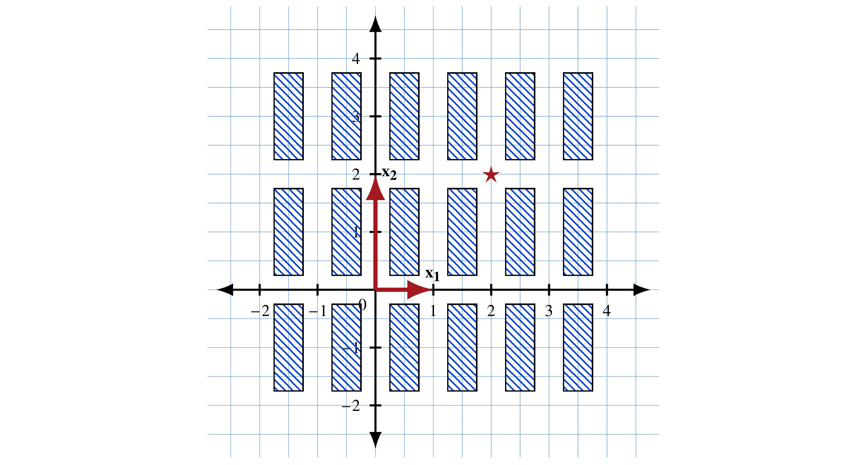
We are familiar with many properties of objects, such as lines and circles in two dimensions, and cubes and spheres in three dimensions. If I ask you how long something is, you might take out a ruler or a tape measure. When you take a photo, you rotate your camera or phone in three dimensions without thinking too much about it.

Alas, there is math behind all these actions. The notion of something existing in one or more dimensions, indeed even the idea of what a dimension is, must be made more formal if we are to perform calculations. This is the concept of vector spaces. The study of what they are and what you can do with them is linear algebra.

Linear algebra is essential to pure and applied mathematics, physics, engineering, and the parts of computer science and software engineering that deal with...

Topics covered in this chapter

1. 5.1. R² and C¹
2. 5.2. Vector spaces
3. 5.3. Linear maps
   1. 5.3.1. Algebraic structure of linear transformations
   2. 5.3.2. Example linear transformations on R²
4. 5.4. Matrices
   1. 5.4.1. Notation and terminology
   2. 5.4.2. Matrices and linear maps
5. 5.5. Matrix algebra
   1. 5.5.1. Arithmetic of general matrices
   2. 5.5.2. Arithmetic of square matrices
6. 5.6. The determinant and trace
7. 5.7. Length and preserving it
   1. 5.7.1. Dot products
   2. 5.7.2. Inner products
   3. 5.7.3. Euclidean norm
   4. 5.7.4. Reflections again
   5. 5.7.5. Projections again
   6. 5.7.6. The Gram-Schmidt orthonormalization process
8. 5.8. Unitary transformations...

5.1 R² and C¹

In section 4.2, we looked at the real plane as a set of standard Cartesian coordinate pairs (x, y) with x and y in R representing points we can plot. We give these pairs an algebraic structure so that if u and v are in R², then so is u + v. Also, if r is in R, we say that r is a scalar. r u and r v are in R² as well. We carry out the addition coordinate by coordinate. The multiplication by r, called scalar multiplication, is also done that way. scalar R² C¹

If u = (u₁, u₂) and v = (v₁, v₂),

Using the origin O = (0, 0) as the identity element, R² is a commutative group under addition. With scalar multiplication by elements of the field R, R² is a two-dimensional vector space over R.

Rather than considering them as pairs or points, we now call u and v vectors. I use bold to indicate a variable or a “point” is a vector. When we plot a vector, we draw it as an arrow from the origin (0, 0) to the point represented...

5.2 Vector spaces

The last section introduced several ideas about vector spaces using familiar notions from R² and C. It’s time to generalize. vector space vector

Let F be a field, for example, Q, R, or C. Let V be a set of objects which we call vectors. We display vectors in bold such as v. F`bold

We are interested in defining vector addition and a special kind of multiplication called scalar multiplication. If s is in F, then we insist s v is in V for all v in V. The set V is closed under multiplication by scalars from the field F. While V may have some kind of multiplication defined between its elements, we do not need to consider it here.

For any v₁ and v₂ in V, we also insist v₁ + v₂ is in V and that the addition is commutative. Thus, V is closed under addition. V must have an identity element 0 and additive inverses so that V is a commutative additive group. group

V is almost a vector space over F, but we insist on a few more...

5.3 Linear maps

We’ve looked at linear functions several times to get a concrete idea of how they work. We must generalize this idea to vector spaces.

Let U and V be vector spaces over the same field F. Let u₁ and u₂ be in U and s₁ and s₂ be scalars in F.

The function L: U → V is a linear map if

In particular, we have

When U = V, we also say L is a linear transformation of U or a linear operator on U. linear$map linear$transformation linear$operator

All linear transformations on R² look like

using Cartesian coordinates, and with a, b, c, d, x, and y in R. This is interesting because the linear transformations on R¹ all look like the somewhat trivial x ↦ ax.

Exercise 5.2

Show that the function

for a, b, c, d, x, and y in C is a linear transformation of C².

The linear transformations on R^3...

5.4 Matrices

If we write out the details of a linear transformation of a five-dimensional vector space over a field F, it looks like this: matrix

This notation is not practical, especially if we start looking at the formulas for compositions of linear maps. Hence, we introduce matrices.

We begin with notation and then move on to the algebra.

5.4.1 Notation and terminology

This array of values with entries in the field F

is a 3-by-4 matrix: it has three rows, four columns, and 12 = 3 × 4 entries. The dimension of this matrix is 3-by-4. matrix$dimension matrix$entry

When we need subscripts for the entries in a matrix, they look like this:

for a 3-by-3 matrix. The first subscript is the row index, and the second is the column index. matrix$row index matrix$column index

In mathematics and physics, we use 1 as the first row or column index. In computer science and...

5.5 Matrix algebra

So far, we have looked at matrices and their relationships to linear maps. We now investigate operations on one or more matrices. We’ll first cover the general case of matrices which may have different numbers of rows and columns, and then move on to square matrices.

All matrices are over fields in this section, and when we manipulate multiple matrices, they all have entries in the same field. We can consider matrices over rings such as the integers, but we do not need to make this restriction for quantum computing.

5.5.1 Arithmetic of general matrices

Matrices of the same size, meaning they have the same number of rows and columns, can be added together entry by entry. For example,

The same is true for subtraction and negation:

We multiply by a scalar entry by entry:

Exercise 5.12

Verify that the set of n-by-m matrices over a field...

5.6 The determinant and trace

Ah, the determinant, a function on square matrices that produces values in F. It’s so elegant, so useful, tells us so much, and is such an annoying and error-prone thing to compute beyond the 2-by-2 case. matrix$determinant determinant

Let’s look at its properties before we discuss its calculation. Let A be an n-by-n matrix. We denote its determinant by det(A):

• det(A) ≠ 0 if and only if A is invertible.
• For b a scalar in F, det(bA) = bⁿ det(A).
• If any row or column of A is all zeros, then det(A) = 0. The determinant being zero does not imply a row or column is zero.
• If A is upper or lower triangular, the determinant is the product of the diagonal entries. If one of those diagonal entries is 0, the determinant is thus 0.
• In particular, det(I) = 1 for I an identity matrix.
• The determinant behaves well when taking transposes and conjugates:

...

5.7 Length and preserving it

Length is a natural notion in the real world, but it needs to be defined precisely in vector spaces. Using complex numbers complicates things because we need to use conjugation. Length is related to magnitude, which measures how big something is. Understanding length and norms is key to the mathematics of quantum algorithms, as we shall see in Chapter 10, “From Circuits to Algorithms.” length

5.7.1 Dot products

Let V be a finite-dimensional vector space over R, and let v = (v₁, v₂, …, v_n) and w = (w₁, w₂, …, w_n) be two vectors in V.

The dot product “·” of v and w is the sum of the products of the corresponding entries in v and w: dot product product$dot ·`strong

If we think of v and w as row vectors and so as 1-by-n matrices, then

The dot product of the basis vectors e₁ = (1, 0) and e₂ = (0, 1) is 0. When this happens...

5.8 Unitary transformations

What are the characteristics of linear transformations that preserve length? If L: V → V and it is always true that ‖L(v)‖ = ‖v‖, what can we say about the matrix of L?

A complex square matrix U is unitary if its adjoint U^† is its inverse U^–1. Hence, U U^† = U^† U = I. The columns of U are orthonormal, as are the rows, which follows from the definition of the complex inner product. matrix$unitary unitary$matrix

For a unitary matrix U, |det(U)| = 1 because

To prove that unitary matrices preserve length, we must do more transposition and conjugation math:

Since the lengths are nonnegative, ‖U v‖ = ‖v‖. Conversely, if this holds, we must have U^† U = I.

Rotations and reflections are unitary. An orthogonal matrix is unitary.

...

5.9 Change of basis

Given an n-dimensional vector space V, we can choose different bases for V. Let’s call two of them basis$change of

If v is a vector in V, it has one set of coordinates corresponding to X and another set for Y. How do we change from one set of coordinates for v to the other?

Let’s look at an example demonstrating how the choice of basis can make things easier.

Suppose we have city blocks laid out in a rectilinear pattern as in Figure 5.20. We use the basis vectors x₁ = (1, 0) and x₂ = (0, 2) to position ourselves. I’ve given the coordinates using the standard basis.

Figure 5.20: City blocks laid out according to the standard basis grid

I can give you directions by saying, “Go north along x₂ for 1 block, turn right, and go east along x₁ for 2 blocks.” That puts you where the star is in the picture. In terms of the X basis, the position is 2x₁ +...

5.10 Eigenvectors and eigenvalues

Let’s review some of the features of diagonal matrices. Recall that a diagonal matrix has 0s everywhere except maybe on the main diagonal. A simple example for R³ is matrix$diagonal matrix$eigenvalue eigenvalue matrix$eigenvector eigenvector

Its effect on the standard basis vectors e₁, e₂, and e₃ is to stretch by a factor of 3 along the first, leave the second alone, reflect across the xy-plane, and then stretch by a factor of 2 along the third.

A general diagonal matrix looks like

Of course, we might be dealing with a small matrix and not have quite so many zeros. Some of the d_j might be zero.

For a diagonal matrix D as above,

• det(D) = d₁ d₂ ⋯ d_n.
• tr (D) = d₁ + d₂ + ⋯ + d_n.
• D^T = D.
• D is invertible if and only if none of the d_j are 0.
• If D is invertible,

• If {b₁, b₂, …...

5.11 Direct sums

Our treatment of vector spaces has alternated between the fairly concrete examples of R² and R³ and the more abstract definition presented in section 5.2. I continue going back and forth with the fundamental idea of the direct sum of two vector spaces over the same field F. direct sum vector space$direct sum ⊕ (direct sum)

In a vague and neither concrete nor abstract sense, a direct sum is when you push two vector spaces together. It’s one of the ways you can construct a new vector space from existing ones.

Let V and W be two vector spaces of dimensions n and m over F. If we write v = (v₁, v₂, …, v_n) and w = (w₁, w₂, …, w_m), then

in the direct sum vector space V ⊕ W. It has dimension n + m.

All the requirements regarding addition and scalar multiplication follow directly from this definition because we perform those operations coordinate by coordinate. We’...

5.12 Homomorphisms

When functions operate on collections with algebraic structure, we usually require additional properties to be preserved. We can now redefine linear maps and transformations of vector spaces in terms of these functions, called homomorphisms. homomorphism

5.12.1 Group homomorphisms

Suppose (G, ★) and (H, •) are groups, which we first explored in section 3.6.1. The function f : G → H is a group homomorphism if for any two elements a and b in G, homomorphism$group group$homomorphism

This means that f is not just a function, but it preserves the operations of the groups.

We have the following properties for group homomorphisms:

• f (id_G) = f (id_G ★ id_G) = f (id_G) • f (id_G), which means f (id_G) = id_H.
• id_H = f (id_G) = f (a ★ a^–1) = f (a) • f (a^–...

5.13 Systems of linear equations

The two equations

together are an example of a system of linear equations. On the left of the equal signs are linear expressions, and on the right are constants. In R², these represent two lines. In general, two lines in R² may be the same, be parallel and so never intersect, or intersect at a single point.

If we use subscripted variables, the same relationship might be expressed by

We can further rewrite this in matrix and vector form as

If we let

then our system is simply Ax = b. This is a standard form for writing such systems of any dimension, and we call it a linear equation. linear$equation

Our goal may be to solve for all of x, learn only some of the x_j, or understand some function f applied to x. If A is invertible, then

In this case, there is one possible value for x. If A is not invertible, then there might be no solution or a vector space...

5.14 Summary

Linear algebra is the area of mathematics where we gain the language and tools necessary for understanding and working with spaces of arbitrary dimension. General quantum mechanics in physics uses infinite dimensional spaces. Our needs are simpler, and we focused on vectors, linear transformations, and matrices in finite dimensions.

The fundamental quantum unit of information is the qubit, and its states can be represented in a two-dimensional complex vector space. We now have almost all the tools necessary to jump from the purely mathematical description to one that takes in the evidence from models of the physical world of the very small. One preliminary topic remains, and we tackle that in the next chapter: probability. qubit