Time series decomposition is the process of splitting a time series into its basic components, such as trend or seasonality. This recipe explores different techniques to solve this task and how to choose among them.
Getting ready
A time series is composed of three parts – trend, seasonality, and the remainder:
- The trend characterizes the long-term change in the level of a time series. Trends can be upward (increase in level) or downward (decrease in level), and they can also change over time.
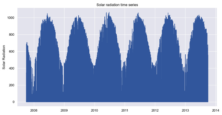
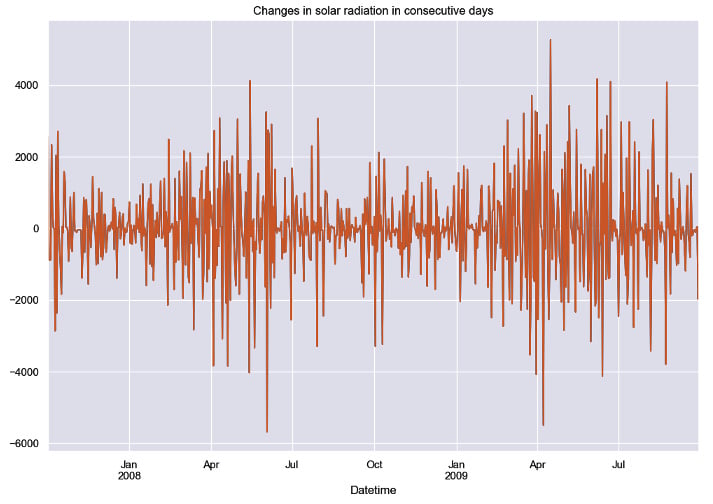
- Seasonality refers to regular variations in fixed periods, such as every day. The solar radiation time series plotted in the preceding recipe shows a clear yearly seasonality. Solar radiation is higher during summer and lower during winter.
- The remainder (also called irregular) of the time series is what is left after removing the trend and seasonal components.
Breaking a time series into its components is useful to understand the underlying structure of the data.
We’ll describe the process of time series decomposition with two methods: the classical decomposition approach and a method based on local regression. You’ll also learn how to extend the latter method to time series with multiple seasonal patterns.
How to do it…
There are several approaches for decomposing a time series into its basic parts. The simplest method is known as classical decomposition. This approach is implemented in the statsmodels library and can be used as follows:
from statsmodels.tsa.seasonal import seasonal_decompose
result = seasonal_decompose(x=series_daily,
                            model='additive',
                            period=365)
Besides the dataset, you need to specify the period and the type of model. For a daily time series with a yearly seasonality, the period should be set to 365, which is the number of days in a year. The model parameter can be either additive or multiplicative. We’ll go into more detail about this in the next section.
Each component is stored as an attribute of the results in an object:
result.trend
result.seasonal
result.resid
Each of these attributes returns a time series with the respective component.
Arguably, one of the most popular methods for time series decomposition is STL (which stands for Seasonal and Trend decomposition using LOESS). This method is also available on statsmodels:
from statsmodels.tsa.seasonal import STL
result = STL(endog=series_daily, period=365).fit()
In the case of STL, you don’t need to specify a model as we did with the classical method.
Usually, time series decomposition approaches work under the assumption that the dataset contains a single seasonal pattern. Yet, time series collected in high sampling frequencies (such as hourly or daily) can contain multiple seasonal patterns. For example, an hourly time series can show both regular daily and weekly variations.
The MSTL() method (short for Multiple STL) extends MSTL for time series with multiple seasonal patterns. You can specify the period for each seasonal pattern in a tuple as the input for the period argument. An example is shown in the following code:
from statsmodels.tsa.seasonal import MSTL
result = MSTL(endog=series_daily, periods=(7, 365)).fit()
In the preceding code, we passed two periods as input: 7 and 365. These periods attempt to capture weekly and yearly seasonality in a daily time series.
How it works…
In a given time step i, the value of the time series (Yi) can be decomposed using an additive model, as follows:
Yi = Trendi+Seasonalityi+Remainderi
This decomposition can also be multiplicative:
Yi = Trendi×Seasonalityi×Remainderi
The most appropriate approach, additive or multiplicative, depends on the input data. But you can turn a multiplicative decomposition into an additive one by transforming the data with the logarithm function. The logarithm stabilizes the variance, thus making the series additive regarding its components.
The results of the classical decomposition are shown in the following figure:
Figure 1.3: Time series components after decomposition with the classical method
In the classical decomposition, the trend is estimated using a moving average, for example, the average of the last 24 hours (for hourly series). Seasonality is estimated by averaging the values of each period. STL is a more flexible method for decomposing a time series. It can handle complex patterns, such as irregular trends or outliers. STL leverages LOESS, which stands for locally weighted scatterplot smoothing, to extract each component.
There’s more…
Decomposition is usually done for data exploration purposes. But it can also be used as a preprocessing step for forecasting. For example, some studies show that removing seasonality before training a neural network improves forecasting performance.
See also
You can learn more about this in the following references:
- Hewamalage, Hansika, Christoph Bergmeir, and Kasun Bandara. “Recurrent neural networks for time series forecasting: Current status and future directions.” International Journal of Forecasting 37.1 (2021): 388-427.
- Hyndman, Rob J., and George Athanasopoulos. Forecasting: Principles and Practice. OTexts, 2018.
 Argentina
 Australia
 Austria
 Belgium
 Brazil
 Bulgaria
 Canada
 Chile
Chile
 Colombia
 Cyprus
 Czechia
 Denmark
 Ecuador
 Egypt
Egypt
 Estonia
 Finland
 France
 Germany
 Great Britain
 Greece
 Hungary
 India
India
 Indonesia
 Ireland
 Italy
Italy
 Japan
Japan
 Latvia
 Lithuania
 Luxembourg
 Malaysia
 Malta
Malta
 Mexico
 Netherlands
 New Zealand
 Norway
 Philippines
 Poland
 Portugal
 Romania
 Russia
 Singapore
 Slovakia
 Slovenia
 South Africa
 South Korea
 Spain
Spain
 Sweden
 Switzerland
 Taiwan
 Thailand
 Turkey
 Ukraine
 United States