Welcome to the fantastic world of data! Are you ready to embark on a thrilling journey into data ingestion? If so, this is the perfect book to start! Ingesting data is the first step into the big data world.

Data ingestion is a process that involves gathering and importing data and also storing it properly so that the subsequent extract, transform, and load (ETL) pipeline can utilize the data. To make it happen, we must be cautious about the tools we will use and how to configure them properly.

In our book journey, we will use Python and PySpark to retrieve data from different data sources and learn how to store them properly. To orchestrate all this, the basic concepts of Airflow will be implemented, along with efficient monitoring to guarantee that our pipelines are covered.

This chapter will introduce some basic concepts about data ingestion and how to set up your environment to start the tasks.

In this chapter, you will build and learn the following recipes:

• Setting up Python and the environment
• Installing PySpark
• Configuring Docker for MongoDB
• Configuring Docker for Airflow
• Logging libraries
• Creating schemas
• Applying data governance in ingestion
• Implementing data replication

The commands inside the recipes of this chapter use Linux syntax. If you don’t use a Linux-based system, you may need to adapt the commands:

• Docker or Docker Desktop
• The SQL client of your choice (recommended); we recommend DBeaver, since it has a community-free version

You can find the code from this chapter in this GitHub repository: https://github.com/PacktPublishing/Data-Ingestion-with-Python-Cookbook.

Note

Windows users might get an error message such as Docker Desktop requires a newer WSL kernel version. This can be fixed by following the steps here: https://docs.docker.com/desktop/windows/wsl/.

In the data world, languages such as Java, Scala, or Python are commonly used. The first two languages are used due to their compatibility with the big data tools environment, such as Hadoop and Spark, the central core of which runs on a Java Virtual Machine (JVM). However, in the past few years, the use of Python for data engineering and data science has increased significantly due to the language’s versatility, ease of understanding, and many open source libraries built by the community.

Getting ready

Let’s create a folder for our project:

1. First, open your system command line. Since I use the Windows Subsystem for Linux (WSL), I will open the WSL application.
2. Go to your home directory and create a folder as follows:

   $ mkdir my-project

3. Go inside this folder:

   $ cd my-project

4. Check your Python version on your operating system as follows:

   $ python -–version

Depending on your operational system, you might or might not have output here – for example, WSL 20.04 users might have the following output:

Command 'python' not found, did you mean:
 command 'python3' from deb python3
 command 'python' from deb python-is-python3

If your Python path is configured to use the python command, you will see output similar to this:

Python 3.9.0

Sometimes, your Python path might be configured to be invoked using python3. You can try it using the following command:

$ python3 --version

The output will be similar to the python command, as follows:

Python 3.9.0

5. Now, let’s check our pip version. This check is essential, since some operating systems have more than one Python version installed:

   $ pip --version

You should see similar output:

pip 20.0.2 from /usr/lib/python3/dist-packages/pip (python 3.9)

If your operating system (OS) uses a Python version below 3.8x or doesn’t have the language installed, proceed to the How to do it steps; otherwise, you are ready to start the following Installing PySpark recipe.

How to do it…

We are going to use the official installer from Python.org. You can find the link for it here: https://www.python.org/downloads/:

Note

For Windows users, it is important to check your OS version, since Python 3.10 may not be yet compatible with Windows 7, or your processor type (32-bits or 64-bits).

1. Download one of the stable versions.

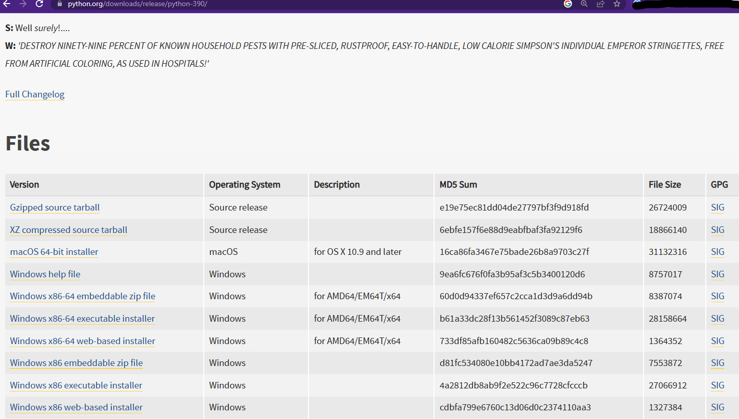
At the time of writing, the stable recommended versions compatible with the tools and resources presented here are 3.8, 3.9, and 3.10. I will use the 3.9 version and download it using the following link: https://www.python.org/downloads/release/python-390/. Scrolling down the page, you will find a list of links to Python installers according to OS, as shown in the following screenshot.

Figure 1.1 – Python.org download files for version 3.9

2. After downloading the installation file, double-click it and follow the instructions in the wizard window. To avoid complexity, choose the recommended settings displayed.

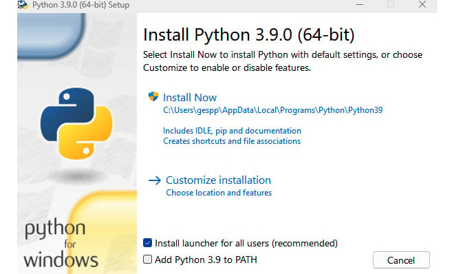
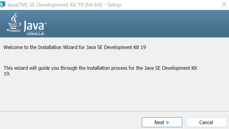
The following screenshot shows how it looks on Windows:

Figure 1.2 – The Python Installer for Windows

3. If you are a Linux user, you can install it from the source using the following commands:

   $ wget https://www.python.org/ftp/python/3.9.1/Python-3.9.1.tgz
   $ tar -xf Python-3.9.1.tgz
   $ ./configure –enable-optimizations
   $ make -j 9

After installing Python, you should be able to execute the pip command. If not, refer to the pip official documentation page here: https://pip.pypa.io/en/stable/installation/.

How it works…

Python is an interpreted language, and its interpreter extends several functions made with C or C++. The language package also comes with several built-in libraries and, of course, the interpreter.

The interpreter works like a Unix shell and can be found in the usr/local/bin directory: https://docs.python.org/3/tutorial/interpreter.html.

Lastly, note that many Python third-party packages in this book require the pip command to be installed. This is because pip (an acronym for Pip Installs Packages) is the default package manager for Python; therefore, it is used to install, upgrade, and manage the Python packages and dependencies from the Python Package Index (PyPI).

There’s more…

Even if you don’t have any Python versions on your machine, you can still install them using the command line or HomeBrew (for macOS users). Windows users can also download them from the MS Windows Store.

Note

If you choose to download Python from the Windows Store, ensure you use an application made by the Python Software Foundation.

See also

You can use pip to install convenient third-party applications, such as Jupyter. This is an open source, web-based, interactive (and user-friendly) computing platform, often used by data scientists and data engineers. You can install it from the official website here: https://jupyter.org/install.

To process, clean, and transform vast amounts of data, we need a tool that provides resilience and distributed processing, and that’s why PySpark is a good fit. It gets an API over the Spark library that lets you use its applications.

Getting ready

Before starting the PySpark installation, we need to check our Java version in our operational system:

1. Here, we check the Java version:

   $ java -version

You should see output similar to this:

openjdk version "1.8.0_292"
OpenJDK Runtime Environment (build 1.8.0_292-8u292-b10-0ubuntu1~20.04-b10)
OpenJDK 64-Bit Server VM (build 25.292-b10, mixed mode)

If everything is correct, you should see the preceding message as the output of the command and the OpenJDK 18 version or higher. However, some systems don’t have any Java version installed by default, and to cover this, we need to proceed to step 2.

2. Now, we download the Java Development Kit (JDK).

Go to https://www.oracle.com/java/technologies/downloads/, select your OS, and download the most recent version of JDK. At the time of writing, it is JDK 19.

The download page of the JDK will look as follows:

Figure 1.3 – The JDK 19 downloads official web page

Execute the downloaded application. Click on the application to start the installation process. The following window will appear:

Note

Depending on your OS, the installation window may appear slightly different.

Figure 1.4 – The Java installation wizard window

Click Next for the following two questions, and the application will start the installation. You don’t need to worry about where the JDK will be installed. By default, the application is configured, as standard, to be compatible with other tools’ installations.

3. Next, we again check our Java version. When executing the command again, you should see the following version:

   $ java -version
   openjdk version "1.8.0_292"
   OpenJDK Runtime Environment (build 1.8.0_292-8u292-b10-0ubuntu1~20.04-b10)
   OpenJDK 64-Bit Server VM (build 25.292-b10, mixed mode)

How to do it…

Here are the steps to perform this recipe:

1. Install PySpark from PyPi:

   $ pip install pyspark

If the command runs successfully, the installation output’s last line will look like this:

Successfully built pyspark
Installing collected packages: py4j, pyspark
Successfully installed py4j-0.10.9.5 pyspark-3.3.2

2. Execute the pyspark command to open the interactive shell. When executing the pyspark command in your command line, you should see this message:

   $ pyspark
   Python 3.8.10 (default, Jun 22 2022, 20:18:18)
   [GCC 9.4.0] on linux
   Type "help", "copyright", "credits" or "license" for more information.
   22/10/08 15:06:11 WARN Utils: Your hostname, DESKTOP-DVUDB98 resolves to a loopback address: 127.0.1.1; using 172.29.214.162 instead (on interface eth0)
   22/10/08 15:06:11 WARN Utils: Set SPARK_LOCAL_IP if you need to bind to another address
   22/10/08 15:06:13 WARN NativeCodeLoader: Unable to load native-hadoop library for your platform... using builtin-java classes where applicable
   Using Spark's default log4j profile: org/apache/spark/log4j-defaults.properties
   Setting default log level to "WARN".
   To adjust logging level use sc.setLogLevel(newLevel). For SparkR, use setLogLevel(newLevel).
   Welcome to
         ____              __
        / __/__  ___ _____/ /__
       _\ \/ _ \/ _ `/ __/  '_/
      /__ / .__/\_,_/_/ /_/\_\   version 3.1.2
         /_/
   Using Python version 3.8.10 (default, Jun 22 2022 20:18:18)
   Spark context Web UI available at http://172.29.214.162:4040
   Spark context available as 'sc' (master = local[*], app id = local-1665237974112).
   SparkSession available as 'spark'.
   >>>

You can observe some interesting messages here, such as the Spark version and the Python used from PySpark.

3. Finally, we exit the interactive shell as follows:

   >>> exit()
   $

How it works…

As seen at the beginning of this recipe, Spark is a robust framework that runs on top of the JVM. It is also an open source tool for creating resilient and distributed processing output from vast data. With the growth in popularity of the Python language in the past few years, it became necessary to have a solution that adapts Spark to run alongside Python.

PySpark is an interface that interacts with Spark APIs via Py4J, dynamically allowing Python code to interact with the JVM. We first need to have Java installed on our OS to use Spark. When we install PySpark, it already comes with Spark and Py4J components installed, making it easy to start the application and build the code.

There’s more…

Anaconda is a convenient way to install PySpark and other data science tools. This tool encapsulates all manual processes and has a friendly interface for interacting with and installing Python components, such as NumPy, pandas, or Jupyter:

1. To install Anaconda, go to the official website and select Products | Anaconda Distribution: https://www.anaconda.com/products/distribution.
2. Download the distribution according to your OS.

For more detailed information about how to install Anaconda and other powerful commands, refer to https://docs.anaconda.com/.

Using virtualenv with PySpark

It is possible to configure and use virtualenv with PySpark, and Anaconda does it automatically if you choose this type of installation. However, for the other installation methods, we need to make some additional steps to make our Spark cluster (locally or on the server) run it, which includes indicating the virtualenv /bin/ folder and where your PySpark path is.

See also

There is a nice article about this topic, Using VirtualEnv with PySpark, by jzhang, here: https://community.cloudera.com/t5/Community-Articles/Using-VirtualEnv-with-PySpark/ta-p/245932.

MongoDB is a Not Only SQL (NoSQL) document-oriented database, widely used to store Internet of Things (IoT) data, application logs, and so on. A NoSQL database is a non-relational database that stores unstructured data differently from relational databases such as MySQL or PostgreSQL. Don’t worry too much about this now; we will cover it in more detail in Chapter 5.

Your cluster production environment can handle huge amounts of data and create resilient data storage.

Getting ready

Following the good practice of code organization, let’s start creating a folder inside our project to store the Docker image:

Create a folder inside our project directory to store the MongoDB Docker image and data as follows:

my-project$ mkdir mongo-local
my-project$ cd mongo-local

How to do it…

Here are the steps to try out this recipe:

1. First, we pull the Docker image from Docker Hub as follows:

   my-project/mongo-local$ docker pull mongo

You should see the following message in your command line:

Using default tag: latest
latest: Pulling from library/mongo
(...)
bc8341d9c8d5: Pull complete
(...)
Status: Downloaded newer image for mongo:latest
docker.io/library/mongo:latest

Note

If you are a WSL user, an error might occur if you use the WSL 1 version instead of version 2. You can easily fix this by following the steps here: https://learn.microsoft.com/en-us/windows/wsl/install.

2. Then, we run the MongoDB server as follows:

   my-project/mongo-local$ docker run \
   --name mongodb-local \
   -p 27017:27017 \
   -e MONGO_INITDB_ROOT_USERNAME="your_username" \
   -e MONGO_INITDB_ROOT_PASSWORD="your_password"\
   -d mongo:latest

We then check our server. To do this, we can use the command line to see which Docker images are running:

my-project/mongo-local$ docker ps

We then see this on the screen:

Figure 1.5 – MongoDB and Docker running container

We can even check on the Docker Desktop application to see whether our container is running:

Figure 1.6 – The Docker Desktop vision of the MongoDB container running

3. Finally, we need to stop our container. We need to use Container ID to stop the container, which we previously saw when checking the Docker running images. We will rerun it in Chapter 5:

   my-project/mongo-local$ docker stop 427cc2e5d40e

How it works…

MongoDB’s architecture uses the concept of distributed processing, where the main node interacts with clients’ requests, such as queries and document manipulation. It distributes the requests automatically among its shards, which are a subset of a larger data collection here.

Figure 1.7 – MongoDB architecture

Since we may also have other running projects or software applications inside our machine, isolating any database or application server used in development is a good practice. In this way, we ensure nothing interferes with our local servers, and the debug process can be more manageable.

This Docker image setting creates a MongoDB server locally and even allows us to make additional changes if we want to simulate any other scenario for testing or development.

The commands we used are as follows:

• The --name command defines the name we give to our container.
• The -p command specifies the port our container will open so that we can access it via localhost:27017.
• -e command defines the environment variables. In this case, we set the root username and password for our MongoDB container.
• -d is detached mode – that is, the Docker process will run in the background, and we will not see input or output. However, we can still use docker ps to check the container status.
• mongo:latest indicates Docker pulling this image’s latest version.

There’s more…

For frequent users, manually configuring other parameters for the MongoDB container, such as the version, image port, database name, and database credentials, is also possible.

A version of this image with example values is also available as a docker-compose file in the official documentation here: https://hub.docker.com/_/mongo.

The docker-compose file for MongoDB looks similar to this:

# Use your own values for username and password
version: '3.1'
services:
  mongo:
    image: mongo
    restart: always
    environment:
      MONGO_INITDB_ROOT_USERNAME: root
      MONGO_INITDB_ROOT_PASSWORD: example
  mongo-express:
    image: mongo-express
    restart: always
    ports:
      - 8081:8081
    environment:
      ME_CONFIG_MONGODB_ADMINUSERNAME: root
      ME_CONFIG_MONGODB_ADMINPASSWORD: example
      ME_CONFIG_MONGODB_URL: mongodb://root:example@mongo:27017/

See also

You can check out MongoDB at the complete Docker Hub documentation here: https://hub.docker.com/_/mongo.

In this book, we will use Airflow to orchestrate data ingests and provide logs to monitor our pipelines.

Airflow can be installed directly on your local machine and any server using PyPi (https://pypi.org/project/apache-airflow/) or a Docker container (https://hub.docker.com/r/apache/airflow). An official and supported version of Airflow can be found on Docker Hub, and the Apache Foundation community maintains it.

However, there are some additional steps to configure our Airflow. Thankfully, the Apache Foundation also has a docker-compose file that contains all other requirements to make Airflow work. We just need to complete a few more steps.

Getting ready

Let’s start by initializing our Docker application on our machine. You can use the desktop version or the CLI command.

Make sure you are inside your project folder for this. Create a folder to store Airflow internal components and the docker-compose.yaml file:

my-project$ mkdir airflow-local
my-project$ cd airflow-local

How to do it…

1. First, we fetch the docker-compose.yaml file directly from the Airflow official docs:

   my-project/airflow-local$ curl -LfO 'https://airflow.apache.org/docs/apache-airflow/2.3.0/docker-compose.yaml'

You should see output like this:

Figure 1.8 – Airflow container image download progress

Note

Check the most stable version of this docker-compose file when you download it, since new, more appropriate versions may be available after this book is published.

2. Next, we create the dags, logs, and plugins folders as follows:

   my-project/airflow-local$ mkdir ./dags ./logs ./plugins

3. Then, we create and set the Airflow user as follows:

   my-project/airflow-local$ echo -e "AIRFLOW_UID=$(id -u)\nAIRFLOW_GID=0" > .env

Note

If you have any error messages related to the AIRFLOW_UID variable, you can create a .env file in the same folder where your docker-compose.yaml file is and define the variable as AIRFLOW_UID=50000.

4. Then, we initialize the database:

   my-project/airflow-local$ docker-compose up airflow-init

After executing the command, you should see output similar to this:

Creating network "airflow-local_default" with the default driver
Creating volume "airflow-local_postgres-db-volume" with default driver
Pulling postgres (postgres:13)...
13: Pulling from library/postgres
(...)
Status: Downloaded newer image for postgres:13
Pulling redis (redis:latest)...
latest: Pulling from library/redis
bd159e379b3b: Already exists
(...)
Status: Downloaded newer image for redis:latest
Pulling airflow-init (apache/airflow:2.3.0)...
2.3.0: Pulling from apache/airflow
42c077c10790: Pull complete
(...)
Status: Downloaded newer image for apache/airflow:2.3.0
Creating airflow-local_postgres_1 ... done
Creating airflow-local_redis_1    ... done
Creating airflow-local_airflow-init_1 ... done
Attaching to airflow-local_airflow-init_1
(...)
airflow-init_1       | [2022-10-09 09:49:26,250] {manager.py:213} INFO - Added user airflow
airflow-init_1       | User "airflow" created with role "Admin"
(...)
airflow-local_airflow-init_1 exited with code 0

5. Then, we start the Airflow service:

   my-project/airflow-local$ docker-compose up

6. Then, we need to check the Docker processes. Using the following CLI command, you will see the Docker images running:

   my-project/airflow-local$ docker ps

These are the images we see:

Figure 1.9 – The docker ps command output

In the Docker Desktop application, you can also see the same containers running but with a more friendly interface:

Figure 1.10 – A Docker desktop view of the Airflow containers running

7. Then, we access Airflow in a web browser:

In your preferred browser, type http://localhost:8080/home. The following screen will appear:

Figure 1.11 – The Airflow UI login page

8. Then, we log in to the Airflow platform. Since it’s a local application used for testing and learning, the default credentials (username and password) for administrative access in Airflow are airflow.

When logged in, the following screen will appear:

Figure 1.12 – The Airflow UI main page

9. Then, we stop our containers. We can stop our containers until we reach Chapter 9, when we will explore data ingest in Airflow:

   my-project/airflow-local$ docker-compose stop

How it works…

Airflow is an open source platform that allows batch data pipeline development, monitoring, and scheduling. However, it requires other components, such as an internal database, to store metadata to work correctly. In this example, we use PostgreSQL to store the metadata and Redis to cache information.

All this can be installed directly in our machine environment one by one. Even though it seems quite simple, it may not be due to compatibility issues with OS, other software versions, and so on.

Docker can create an isolated environment and provide all the requirements to make it work. With docker-compose, it becomes even simpler, since we can create dependencies between the components that can only be created if the others are healthy.

You can also open the docker-compose.yaml file we downloaded for this recipe and take a look to explore it better. We will also cover it in detail in Chapter 9.

See also

If you want to learn more about how this docker-compose file works, you can look at the Apache Airflow official Docker documentation on the Apache Airflow documentation page: https://airflow.apache.org/docs/apache-airflow/stable/howto/docker-compose/index.html.

Schemas are considered blueprints of a database or table. While some databases strictly require schema definition, others can work without it. However, in some cases, it is advantageous to work with data schemas to ensure that the application data architecture is maintained and can receive the desired data input.

Getting ready

Let’s imagine we need to create a database for a school to store information about the students, the courses, and the instructors. With this information, we know we have at least three tables so far.

Figure 1.13 – A table diagram for three entities

In this recipe, we will cover how schemas work using the Entity Relationship Diagram (ERD), a visual representation of relationships between entities in a database, to exemplify how schemas are connected.

How to do it…

Here are the steps to try this:

1. We define the type of schema. The following figure helps us understand how to go about this:

Figure 1.14 – A diagram to help you decide which schema to use

2. Then, we define the fields and the data type for each table column:

Figure 1.15 – A definition of the columns of each table

3. Next, we define which fields can be empty or NULL:

Figure 1.16 – A definition of which columns can be NULL

4. Then, we create the relationship between the tables:

Figure 1.17 – A relationship diagram of the tables

How it works…

When designing data schemas, the first thing we need to do is define their type. As we can see in the diagram in step 1, applying the schema architecture depends on the data’s purpose.

After that, the tables are designed. Deciding how to define data types can vary, depending project or purpose, but deciding what values a column can receive is important. For instance, the officeRoom on Teacher table can be an Integer type if we know the room’s identification is always numeric, or a String type if it is unsure how identifications are made (for example, Room 3-D).

Another important topic covered in step 3 is how to define which of the columns can accept NULL fields. Can a field for a student’s name be empty? If not, we need to create a constraint to forbid this type of insert.

Finally, based on the type of schema, a definition of the relationship between the tables is made.

See also

If you want to know more about database schema designs and their application, read this article by Mark Smallcombe: https://www.integrate.io/blog/database-schema-examples/.

Data governance is a set of methodologies that ensure that data is secure, available, well-stored, documented, private, and accurate.

Getting ready

Data ingestion is the beginning of the data pipeline process, but it doesn’t mean data governance is not heavily applied. The governance status in the final data pipeline output depends on how it was implemented during the ingestion.

The following diagram shows how data ingestion is commonly conducted:

Figure 1.18 – The data ingestion process

Let’s analyze the steps in the diagram:

1. Getting data from the source: The first step is to define the type of data, its periodicity, where we will gather it, and why we need it.
2. Writing the scripts to ingest data: Based on the answers to the previous step, we can begin planning how our code will behave and some basic steps.
3. Storing data in a temporary database or other types of storage: Between the ingest and the transformation phase, data is typically stored in a temporary database or repository.

Figure 1.19 – Data governance pillars

How to do it…

Step by step, let’s attribute the pillars in Figure 1.19 to the ingestion phase:

1. A concern for accessibility needs to be applied at the data source level, defining the individuals that are allowed to see or retrieve data.
2. Next, it is necessary to catalog our data to understand it better. Since data ingestion is only covered here, it is more relevant to cover the data sources.
3. The quality pillar will be applied to the ingestion and staging area, where we control the data and keep its quality aligned with the source.
4. Then, let’s define ownership. We know the data source belongs to a business area or a company. However, when we ingested the data and put it in temporary or staging storage, it becomes our responsibility to maintain it.
5. The last pillar involves keeping data secure for the whole pipeline. Security is vital in all steps, since we may be handling private or sensitive information.

Figure 1.20 – Adding to data ingestion

How it works…

While some articles define “pillars” to create governance good practices, the best way to understand how to apply them is to understand how they are composed. As you saw in the previous How to do it… section, we attributed some items to our pipeline, and now we can understand how they are connected to the following topics:

• Data accessibility: Data accessibility is how people from a group, organization, or project can see and use data. The information needs to be readily available for use. At the same time, it needs to be available for the people involved in the process. For example, sensitive data accessibility should be restricted to some people or programs. In the diagram we built, we applied it to our data sources, since we need to understand and retrieve data. For the same reason, it can be applied for temporary storage needs as well.
• Data catalog: Cataloging and documenting data are essential for business and engineering teams. When we know what types of information rely on our databases or data lakes and have quick access to these documents, the action time to solve a problem becomes short.

Again, documenting our data sources can make the ingest process quicker, since we need to make a discovery every time we need to ingest data.

• Data quality: Quality is constantly preoccupied with ingesting, processing, and loading data. Tracking and monitoring data’s expected income and outcome by its periodicity is essential. For example, if we expect to ingest 300 GB of data per day and suddenly it drops to 1 GB, something is very wrong and will affect the quality of our final output. Other quality parameters can be the number of columns, partitioning, and so on, which we will explore later in this book.
• Ownership: Who is responsible for the data? This definition is crucial to make contact with the owner if there are problems or attribute responsibility to keep and maintain data.
• Security: A concerning topic nowadays is data security. With so many regulations about data privacy, it became an obligation of data engineers and scientists to know, at least, the basics of encryption, sensitive data, and how to avoid data leaks. Even languages and libraries that are used for work need to be evaluated. That’s why this item is attributed to the three steps in Figure 1.19.

In addition to the topics we explored, a global data governance project has a vital role called a data steward, which is responsible for managing an organization’s data assets and ensuring that data is accurate, consistent, and secure. In summary, data stewardship is managing and overseeing an organization’s data assets.

See also

You can read more about a recent vulnerability found in one of the most used tools for data engineering here: https://www.ncsc.gov.uk/information/log4j-vulnerability-what-everyone-needs-to-know.

Data replication is a process applied in data environments to create multiple copies of data and store them on different locations, servers, or sites. This technique is commonly implemented to create better availability and avoid data loss if there is downtime, or even a natural disaster that affects a data center.

Getting ready

You will find across papers and articles different types (or even names) on the best way for data replication decision. In this recipe, you will learn how to decide which kind of replication better suits your application or software.

How to do it…

Let’s begin to build our fundamental pillars to implement data replication:

1. First, we need to decide the size of our replication, and it can be done using a portion or all the stored data.
2. The next step is to consider when replication will take place. It can be done synchronously when new data arrives in storage or within a specific timeframe.
3. The last fundamental pillar is whether the data is incremented or in a bulk form.

In the end, we will have a diagram that looks like the following:

Figure 1.21 – A data replication model decision diagram

How it works…

Analyzing the preceding figure, we have three main questions to answer, regarding the extension, the frequency, and whether our replication will be incremental or bulk.

For the first question, we decide whether the replication will be complete or partial. In other words, either the data will consistently be replicated no matter what type of transaction or change was made, or just a portion of the data will be replicated. A real example of this would be keeping track of all store sales or just the most expensive ones.

The second question, related to the frequency, is to decide when a replication needs to be done. This question also needs to take into consideration related costs. Real-time replication is often more expensive, but the synchronicity guarantees almost no data inconsistency.

Lastly, it is relevant to consider how data will be transported to the replication site. In most cases, a scheduler with a script can replicate small data batches and reduce transportation costs. However, a bulk replication can be used in the data ingestion process, such as copying all the current batch’s raw data from a source to cold storage.

There’s more…

One method of data replication that has seen an increase in use in the past few years is cold storage, which is used to retain data used infrequently or is even inactive. The costs related to this type of replication are meager and guarantee data longevity. You can find cold storage solutions in all cloud providers, such as Amazon Glacier, Azure Cool Blob, and Google Cloud Storage Nearline.

Besides replication, regulatory compliance such as General Data Protection Regulation (GDPR) laws benefit from this type of storage, since, for some case scenarios, users’ data need to be kept for some years.

In this chapter, we explored the basic concepts and laid the foundation for the following chapters and recipes in this book. We started with a Python installation, prepared our Docker containers, and saw data governance and replication concepts. You will observe over the upcoming chapters that almost all topics interconnect, and you will understand the relevance of understanding them at the beginning of the ETL process.

• https://www.manageengine.com/device-control/data-replication.html