Chapter 6. Neural Networks

Artificial neural networks, as the name suggests, are based algorithms that attempt to mimic the way neurons work in the brain. Conceptual work began in the 1940s, but it is only somewhat recently that a number of important insights, together with the availability of hardware to run these more computationally expensive models, have given neural networks practical application. They are now state-of-the-art techniques that are at the heart of many advanced machine learning applications.

In this chapter, we will introduce the following topics:

• Logistic units

• The cost function for neural networks

• Implementing a neural network

• Other neural network architectures

Getting started with neural networks

We saw in the last chapter how we could create a nonlinear decision boundary by adding polynomial terms to our hypothesis function. We can also use this technique in linear regression to fit nonlinear data. However, this is not the ideal solution for a number of reasons. Firstly, we have to choose polynomial terms, and for complicated decision boundaries, this can be an imprecise and time-intensive process, which can take quite a bit of trial and error. We also need to consider what happens when we have a large number of features. It becomes difficult to understand exactly how added polynomial terms will change the decision boundary. It also means that the possible number of derived features will grow exponentially. To fit complicated boundaries, we will need many higher-order terms, and our model will become unwieldy, computationally expensive, and hard to understand.

Consider applications such as computer vision, where in a gray scale image, each pixel...

Logistic units

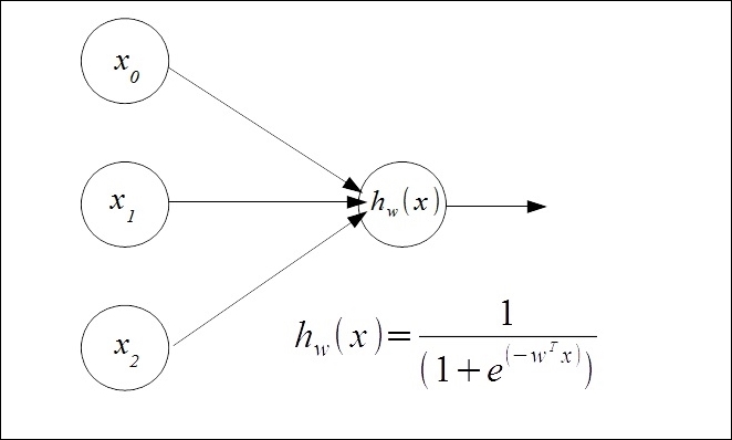
As a starting point, we use the idea of a logistic unit over the simplified model of a neuron. It consists of a set of inputs and outputs and an activation function. This activation function is essentially performing a calculation on the set of inputs, and subsequently giving an output. Here, we set the activation function to the sigmoid that we used for logistic regression in the previous chapter:

We have Two input units, x₁ and x₂ and a bias unit, x₀, that is set to one. These are fed into a hypothesis function that uses the sigmoid logistic function and a weight vector, w, which parameterizes the hypothesis function. The feature vector, consisting of binary values, and the parameter vector for the preceding example consist of the following:

To see how we can get this to perform logical functions, let's give the model some weights. We can write this as a function of the sigmoid, g, and our weights. To get started, we are just going to choose some weights. We will learn shortly...

Cost function

To fit the weights in a neural net for a given training set, we first need to define a cost function:

This is very similar to the cost function we used for logistic regression, except that now we are also summing over k output units. The triple summation used in the regularization term looks a bit complicated, but all it is really doing is summing over each of the terms in the parameter matrix, and using this to calculate the regularization. Note that the summation, i, l, and j start at 1, rather than 0; this is to reflect the fact that we do not apply regularization to the bias unit.

Minimizing the cost function

Now that we have cost function, we need to work out a way to minimize it. As with gradient descent, we need to compute the partial derivatives to calculate the slope of the cost function. This is done using the back propagation algorithm. It is called back propagation because we begin by calculating the error at the output layer, then calculating the error for each previous...

Implementing a neural network

There is one more thing we need to consider, and that is the initialization of our weights. If we initialize them to 0, or all to the same number, all the units on the forward layer will be computing the same function at the input, making the calculation highly redundant and unable to fit complex data. In essence, what we need to do is break the symmetry so that we give each unit a slightly different starting point that actually allows the network to create more interesting functions.

Now, let's look at how we might implement this in code. This implementation is written by Sebastian Raschka, taken from his excellent book, Python Machine Learning, released by Packt Publishing:

import numpy as np
from scipy.special import expit
import sys


class NeuralNetMLP(object):
  
    def __init__(self, n_output, n_features, n_hidden=30,
                 l1=0.0, l2=0.0, epochs=500, eta=0.001, 
                 alpha=0.0, decrease_const=0.0, shuffle=True,
               ...

Gradient checking

Back propagation, and neural nets in general, are a little difficult to conceptualize. So, it is often not easy to understand how changing any of the model (hyper) parameters will affect the outcome. Furthermore, with different implementations, it is possible to get results that indicate that an algorithm is working correctly, that is, the cost function is decreasing on each level of gradient descent. However, as with any complicated software, there can be hidden bugs that might only manifest themselves under very specific conditions. A way to help eliminate these is through a procedure called gradient checking. This is a numerical way of approximating gradients, and we can understand this intuitively by examining the following diagram:

The derivative of J(w), with respect to w, can be approximated as follows:

The preceding formula approximates the derivative when the parameter is a single value. We need to evaluate these derivatives on a cost function, where the weights...

Other neural net architectures

Much of the most important work being done in the field of neural net models, and indeed machine learning in general, is using very complex neural nets with many layers and features. This approach is often called deep architecture or deep learning. Human and animal learning occurs at a rate and depth that no machine can match. Many of the elements of biological learning still remain a mystery. One of the key areas of research, and one of the most useful in practical applications, is that of object recognition. This is something quite fundamental to living systems, and higher animals have evolved an extraordinary ability to learn complex relationships between objects. Biological brains have many layers; each synaptic event exists in a long chain of synaptic processes. In order to recognize complex objects, such as people's faces or handwritten digits, a fundamental task that is needed is to create a hierarchy of representation from the raw input to higher and...

Summary

In this chapter, we introduced the powerful machine learning algorithms of artificial neural networks. We saw how these networks are a simplified model of neurons in the brain. They can perform complex learning tasks, such as learning highly nonlinear decision boundaries, using layers of artificial neurons, or units, to learn new features from labelled data. In the next chapter, we will look at the crucial component of any machine learning algorithm, that is, its features.