Chapter 1. Python and the Surrounding Software Ecology

In this chapter, we will cover the following recipes:

Installing the required software with Anaconda
Installing the required software with Docker
Interfacing with R via rpy2
Performing R magic with Jupyter Notebook

Introduction

We will start by installing the required software. This will include the Python distribution, some fundamental Python libraries, and external bioinformatics software. Here, we will also be concerned with the world outside Python. In bioinformatics and big data, R is also a major player; therefore, you will learn how to interact with it via rpy2, which is a Python/R bridge. We will also explore the advantages that the IPython framework (via Jupyter Notebook) can give us in order to efficiently interface with R. This chapter will set the stage for all of the computational biology that we will perform in the rest of this book.

As different users have different requirements, we will cover two different approaches for installing the software. One approach is using the Anaconda Python (http://docs.continuum.io/anaconda/) distribution, and another approach to install the software is via Docker (a server virtualization method based on containers sharing the same operating system kernel—https://www.docker.com/). If you are using a Windows-based operating system, you are strongly encouraged to consider changing your operating system or use Docker via some of the existing options on Windows. On macOS, you might be able to install most of the software natively, though Docker is also available.

Installing the required software with Anaconda

Before we get started, we need to install some prerequisite software. The following sections will take you through the software and the steps needed to install them. An alternative way to start is to use the Docker recipe, after which everything will be taken care for you via a Docker container.

If you are already using a different Python version, you are strongly encouraged to consider Anaconda, as it has become the de facto standard for data science. Also, it is the distribution that will allow you to install software from Bioconda (https://bioconda.github.io/).

Getting ready

Python can be run on top of different environments. For instance, you can use Python inside the Java Virtual Machine (JVM) (via Jython) or with .NET (with IronPython). However, here, we are concerned not only with Python, but also with the complete software ecology around it; therefore, we will use the standard (CPython) implementation, since the JVM and .NET versions exist mostly to interact with the native libraries of these platforms. A potentially viable alternative would be to use the PyPy implementation of Python (not to be confused with Python Package Index (PyPI).

Save for noted exceptions, we will be using Python 3 only. If you were starting with Python and bioinformatics, any operating system will work, but here, we are mostly concerned with intermediate to advanced usage. So, while you can probably use Windows and macOS, most heavy-duty analysis will be done on Linux (probably on a Linux cluster). Next-generation sequencing (NGS) data analysis and complex machine learning is mostly performed on Linux clusters.

If you are on Windows, you should consider upgrading to Linux for your bioinformatics work because most modern bioinformatics software will not run on Windows. macOS will be fine for almost all analyses, unless you plan to use a computer cluster, which will probably be Linux-based.

If you are on Windows or macOS and do not have easy access to Linux, don't worry. Modern virtualization software (such as VirtualBox and Docker) will come to your rescue, which will allow you to install a virtual Linux on your operating system. If you are working with Windows and decide that you want to go native and not use Anaconda, be careful with your choice of libraries; you are probably safer if you install the 32-bit version for everything (including Python itself).

Note

If you are on Windows, many tools will be unavailable to you.

Note

Bioinformatics and data science are moving at breakneck speed; this is not just hype, it's a reality. When installing software libraries, choosing a version might be tricky. Depending on the code that you have, it might not work with some old versions, or maybe not even work with a newer version. Hopefully, any code that you use will indicate the correct dependencies—though this is not guaranteed.

The software developed for this book is available at https://github.com/PacktPublishing/Bioinformatics-with-Python-Cookbook-Second-Edition. To access it, you will need to install Git. Alternatively, you can download the ZIP file that GitHub makes available (indeed, getting used to Git may be a good idea because lots of scientific computing software is being developed with it).

Before you install the Python stack properly, you will need to install all the external non-Python software that you will be interoperating with. The list will vary from chapter to chapter, and all chapter-specific packages will be explained in their respective chapters. Some less common Python libraries may also be referred to in their specific chapters. Fortunately, since the first edition of this book, most bioinformatics software can be easily installed with conda using the Bioconda project.

If you are not interested in a specific chapter, you can skip the related packages and libraries. Of course, you will probably have many other bioinformatics applications around—such as Burrows-Wheeler Aligner (bwa) or Genome Analysis Toolkit (GATK) for NGS—but we will not discuss these because we do not interact with them directly (although we might interact with their outputs).

You will need to install some development compilers and libraries, all of which are free. On Ubuntu, consider installing the build-essential package (apt-get it), and on macOS, consider Xcode (https://developer.apple.com/xcode/).

In the following table, you will find a list of the most important Python software:

Name	Application	URL	Purpose
Project Jupyter	All chapters	https://jupyter.org/	Interactive computing
pandas	All chapters	https://pandas.pydata.org/	Data processing
NumPy	All chapters	http://www.numpy.org/	Array/matrix processing
SciPy	All chapters	https://www.scipy.org/	Scientific computing
Biopython	All chapters	https://biopython.org/	Bioinformatics library
PyVCF	NGS	https://pyvcf.readthedocs.io	VCF processing
Pysam	NGS	https://github.com/pysam-developers/pysam	SAM/BAM processing
HTSeq	NGS/Genomes	https://htseq.readthedocs.io	NGS processing
simuPOP	Population genetics	http://simupop.sourceforge.net/	Population genetics simulation
DendroPY	Phylogenetics	https://dendropy.org/	Phylogenetics
scikit-learn	Machine learning/population genetics	http://scikit-learn.org	Machine learning library
PyMol	Proteomics	https://pymol.org	Molecular visualization
rpy2	Introduction	https://rpy2.readthedocs.io	R interface
seaborn	All chapters	http://seaborn.pydata.org/	Statistical chart library
Cython	Big data	http://cython.org/	High performance
Numba	Big data	https://numba.pydata.org/	High performance
Dask	Big data	http://dask.pydata.org	Parallel processing

We have taken a somewhat conservative approach in most of the recipes with regard to the processing of tabled data. While we use pandas every now and then, most of the time, we use standard Python. As time advances and pandas becomes more pervasive, it will probably make sense to just process all tabular data with it (if it fits in-memory).

How to do it...

Take a look at the following steps to get started:

Start by downloading the Anaconda distribution from https://www.anaconda.com/download. Choose Python version 3. In any case, this is not fundamental, because Anaconda will let you use Python 2 if you need it. You can accept all the installation defaults, but you may want to make sure that the conda binaries are in your path (do not forget to open a new window so that the path is updated). If you have another Python distribution, be careful with your PYTHONPATH and existing Python libraries. It's probably better to unset your PYTHONPATH. As much as possible, uninstall all other Python versions and installed Python libraries.
Let's go ahead with the libraries. We will now create a newcondaenvironment calledbioinformaticswithbiopython=1.70, as shown in the following command:

conda create -n bioinformatics biopython biopython=1.70

Let's activate the environment, as follows:

source activate bioinformatics

Let's add the bioconda and conda-forge channel to our source list:

condaconfig--addchannelsbioconda
condaconfig--addchannelsconda-forge

Also, install the core packages:

conda install scipy matplotlib jupyter-notebook pip pandas cython numba scikit-learn seaborn pysam pyvcf simuPOP dendropy rpy2

Some of them will probably be installed with the core distribution anyway.

We can even install R from conda:

conda install r-essentials r-gridextra

r-essentials installs a lot of R packages, including ggplot2, which we will use later. We also install r-gridextra, since we will be using it in the Notebook.

There's more...

Compared to the first edition of this book, this recipe is now highly simplified. There are two main reasons for this: the bioconda package, and the fact that we only need to support Anaconda as it has become a standard. If you feel strongly against using Anaconda, you will be able to install many of the Python libraries via pip. You will probably need quite a few compilers and build tools—not only C compilers, but also C++ and Fortran.

Installing the required software with Docker

Docker is the most widely-used framework for implementing operating system-level virtualization. This technology allows you to have an independent container: a layer that is lighter than a virtual machine, but still allows you to compartmentalize software. This mostly isolates all processes, making it feel like each container is a virtual machine. Docker works quite well at both extremes of the development spectrum: it's an expedient way to set up the content of this book for learning purposes, and may become your platform of choice for deploying your applications in complex environments. This recipe is an alternative to the previous recipe.

However, for long-term development environments, something along the lines of the previous recipe is probably your best route, although it can entail a more laborious initial setup.

Getting ready

If you are on Linux, the first thing you have to do is install Docker. The safest solution is to get the latest version from https://www.docker.com/. While your Linux distribution may have a Docker package, it may be too old and buggy (remember the "advancing at breakneck speed" thing we mentioned?).

If you are on Windows or macOS, do not despair; take a look at the Docker site. Various options are available there to save you, but there is no clear-cut formula, as Docker advances quite quickly on those platforms. A fairly recent computer is necessary to run our 64-bit virtual machine. If you have any problems, reboot your machine and make sure that on the BIOS, VT-X or AMD-V is enabled. At the very least, you will need 6 GB of memory, preferably more.

Note

This will require a very large download from the internet, so be sure that you have plenty of bandwidth. Also, be ready to wait for a long time.

How to do it...

Follow these steps to get started:

Use the following command on your Docker shell:

docker build -t bio https://raw.githubusercontent.com/PacktPublishing/Bioinformatics-with-Python-Cookbook-Second-Edition/master/docker/Dockerfile

On Linux, you will either need to have root privileges or be added to the Docker Unix group.

Now, you are ready to run the container, as follows:

docker run -ti -p 9875:9875 -v YOUR_DIRECTORY:/data bio

Replace YOUR_DIRECTORY with a directory on your operating system. This will be shared between your host operating system and the Docker container. YOUR_DIRECTORY will be seen in the container on /data and vice versa.-p 9875:9875 will expose the container TCP port 9875 on the host computer port 9875. Especially on Windows (and maybe on macOS), make sure that your directory is actually visible inside the Docker shell environment. If not, check the Docker documentation on how to expose directories.

You are now ready to use the system. Point your browser to http://localhost:9875 and you should get the Jupyter environment.

If this does not work on Windows, check the Docker documentation (https://docs.docker.com/) on how to expose ports.

Interfacing with R via rpy2

If there is some functionality that you need and you cannot find it in a Python library, your first port of call is to check whether it's implemented in R. For statistical methods, R is still the most complete framework; moreover, some bioinformatics functionalities are also only available in R, most probably offered as a package belonging to the Bioconductor project.

rpy2 provides a declarative interface from Python to R. As you will see, you will be able to write very elegant Python code to perform the interfacing process. To show the interface (and try out one of the most common R data structures, the DataFrame, and one of the most popular R libraries, ggplot2), we will download its metadata from the Human 1,000 Genomes Project (http://www.1000genomes.org/). This is not a book on R, but we want to provide interesting and functional examples.

Getting ready

You will need to get the metadata file from the 1,000 Genomes sequence index. Please check https://github.com/PacktPublishing/Bioinformatics-with-Python-Cookbook-Second-Edition/blob/master/Datasets.ipynb and download the sequence.index file. If you are using Jupyter Notebook, open the Chapter01/Interfacing_R.ipynb file and just execute the wget command on top.

This file has information about all of the FASTQ files in the project (we will use data from the Human 1,000 Genomes Project in the chapters to come). This includes the FASTQ file, the sample ID, and the population of origin, and important statistical information per lane, such as the number of reads and number of DNA bases read.

How to do it...

Follow these steps to get started:

Let's start by doing some imports:

import os
from IPython.display import Image
import rpy2.robjects as robjects
import pandas as pd
from rpy2.robjects import pandas2ri
from rpy2.robjects import default_converter
from rpy2.robjects.conversion import localconverter

We will be using pandas on the Python side. R DataFrames map very well to pandas.

We will read the data from our file using R's read.delim function:

read_delim = robjects.r('read.delim')
seq_data = read_delim('sequence.index', header=True, stringsAsFactors=False)
#In R:
# seq.data <- read.delim('sequence.index', header=TRUE, stringsAsFactors=FALSE)

The first thing that we do after importing is access the read.delim R function, which allows you to read files. The R language specification allows you to put dots in the names of objects. Therefore, we have to convert a function name to read_delim. Then, we call the function name proper; note the following highly declarative features. Firstly, most atomic objects, such as strings, can be passed without conversion. Secondly, argument names are converted seamlessly (barring the dot issue). Finally, objects are available in the Python namespace (but objects are actually not available in the R namespace; more about this later).

For reference, I have included the corresponding R code. I hope it's clear that it's an easy conversion. The seq_data object is a DataFrame. If you know basic R or pandas, you are probably aware of this type of data structure; if not, then this is essentially a table: a sequence of rows where each column has the same type.

Let's perform a basic inspection of this DataFrame, as follows:

print('This dataframe has %d columns and %d rows' %
(seq_data.ncol, seq_data.nrow))
print(seq_data.colnames)
#In R:
# print(colnames(seq.data))
# print(nrow(seq.data))
# print(ncol(seq.data))

Again, note the code similarity.

You can even mix styles using the following code:

my_cols = robjects.r.ncol(seq_data)
print(my_cols)

You can call R functions directly; in this case, we will call ncol if they do not have dots in their name; however, be careful. This will display an output, not 26 (the number of columns), but [26], which is a vector that's composed of the element 26. This is because, by default, most operations in R return vectors. If you want the number of columns, you have to perform my_cols[0]. Also, talking about pitfalls, note that R array indexing starts with 1, whereas Python starts with 0.

Now, we need to perform some data cleanup. For example, some columns should be interpreted as numbers, but they are read as strings:

as_integer = robjects.r('as.integer')
match = robjects.r.match

my_col = match('READ_COUNT', seq_data.colnames)[0] # vector returned
print('Type of read count before as.integer: %s' % seq_data[my_col - 1].rclass[0])
seq_data[my_col - 1] = as_integer(seq_data[my_col - 1])
print('Type of read count after as.integer: %s' % seq_data[my_col - 1].rclass[0])

The match function is somewhat similar to the index method in Python lists. As expected, it returns a vector so that we can extract the 0 element. It's also 1-indexed, so we subtract 1 when working on Python. The as_integer function will convert a column into integers. The first print will show strings (values surrounded by " ), whereas the second print will show numbers.

We will need to massage this table a bit more; details on this can be found on the Notebook, but here, we will finalize getting the DataFrame to R (remember that while it's an R object, it's actually visible on the Python namespace):

import rpy2.robjects.lib.ggplot2 as ggplot2

This will create a variable in the R namespace calledseq.data, with the content of the DataFrame from the Python namespace. Note that after this operation, both objects will be independent (if you change one, it will not be reflected on the other).

Note

While you can perform plotting on Python, R has default built-in plotting functionalities (which we will ignore here). It also has a library called ggplot2 that implements the Grammar of Graphics (a declarative language to specify statistical charts).

With regard to our concrete example based on the Human 1,000 Genomes Project, we will first plot a histogram with the distribution of center names, where all sequencing lanes were generated. We will use ggplot for this:

from rpy2.robjects.functions import SignatureTranslatedFunction

ggplot2.theme = SignatureTranslatedFunction(ggplot2.theme, init_prm_translate = {'axis_text_x': 'axis.text.x'})

bar = ggplot2.ggplot(seq_data) + ggplot2.geom_bar() + ggplot2.aes_string(x='CENTER_NAME') + ggplot2.theme(axis_text_x=ggplot2.element_text(angle=90, hjust=1))
robjects.r.png('out.png', type='cairo-png')
bar.plot()
dev_off = robjects.r('dev.off')
dev_off()

The second line is a bit uninteresting, but is an important piece of boilerplate code. One of the R functions that we will call has a parameter with a dot in its name. As Python function calls cannot have this, we must map the axis.text.x R parameter name to the axis_text_r Python name in the function theme. We monkey patch it (that is, we replace ggplot2.theme with a patched version of itself).

We then draw the chart itself. Note the declarative nature of ggplot2 as we add features to the chart. First, we specify the seq_data DataFrame, then we use a histogram bar plot called geom_bar, followed by annotating the x variable (CENTER_NAME). Finally, we rotate the text of the x axis by changing the theme. We finalize this by closing the R printing device.

We can now print the image on the Jupyter Notebook:

Image(filename='out.png')

The following chart is produced:

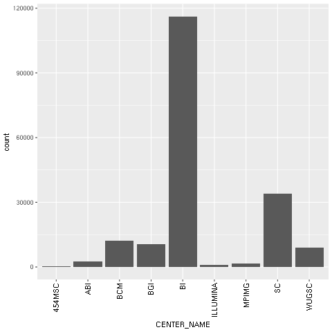
Figure 1: The ggplot2-generated histogram of center names, which is responsible for sequencing the lanes of the human genomic data from the 1,000 Genomes Project

As a final example, we will now do a scatter plot of read and base counts for all the sequenced lanes for Yoruban (YRI) and Utah residents with ancestry from Northern and Western Europe (CEU), using the Human 1,000 Genomes Project (the summary of the data of this project, which we will use thoroughly, can be seen in the Working with modern sequence formats recipe in Chapter 2, Next-Generation Sequencing). We are also interested in the differences between the different types of sequencing (exome, high, and low coverage). First, we generate a DataFrame only just YRI and CEU lanes, and limit the maximum base and read counts:

robjects.r('yri_ceu <- seq.data[seq.data$POPULATION %in% c("YRI", "CEU") & seq.data$BASE_COUNT < 2E9 & seq.data$READ_COUNT < 3E7, ]')
yri_ceu=robjects.r('yri_ceu')

We are now ready to plot:

scatter = ggplot2.ggplot(yri_ceu) + ggplot2.aes_string(x='BASE_COUNT', y='READ_COUNT', shape='factor(POPULATION)', col='factor(ANALYSIS_GROUP)') + ggplot2.geom_point()
robjects.r.png('out.png')
scatter.plot()

Hopefully, this example (refer to the following screenshot) makes the power of the Grammar of Graphics approach clear. We will start by declaring the DataFrame and the type of chart in use (the scatter plot implemented by geom_point).

Note how easy it is to express that the shape of each point depends on the POPULATION variable and the color on the ANALYSIS_GROUP:

Figure 2: The ggplot2-generated scatter plot with base and read counts for all sequencing lanes read; the color and shape of each dot reflects categorical data (population and the type of data sequenced)

Because the R DataFrame is so close to pandas, it makes sense to convert between the two, as that is supported by rpy2:

pd_yri_ceu = pandas2ri.ri2py(yri_ceu)
del pd_yri_ceu['PAIRED_FASTQ']
no_paired = pandas2ri.py2ri(pd_yri_ceu)
robjects.r.assign('no.paired', no_paired)
robjects.r("print(colnames(no.paired))")

We start by importing the necessary conversion module. We then convert the R DataFrame (note that we are converting yri_ceuin the R namespace, not the one on the Python namespace). We delete the column that indicates the name of the paired FASTQ file on the pandas DataFrame and copy it back to the R namespace. If you print the column names of the new R DataFrame, you will see thatPAIRED_FASTQis missing.

There's more...

It's worth repeating that the advances in the Python software ecology are occurring at a breakneck pace. This means that if a certain functionality is not available today, it might be released sometime in the near future. So, if you are developing a new project, be sure to check for the very latest developments on the Python front before using functionality from an R package.

There are plenty of R packages for Bioinformatics in the Bioconductor project (http://www.bioconductor.org/). This should probably be your first port of call in the R world for bioinformatics functionalities. However, note that there are many R Bioinformatics packages that are not on Bioconductor, so be sure to search the wider R packages on Comprehensive R Archive Network (CRAN) (refer to CRAN at http://cran.rproject.org/).

There are plenty of plotting libraries for Python. Matplotlib is the most common library, but you also have a plethora of other choices. In the context of R, it's worth noting that there is a ggplot2-like implementation for Python based on the Grammar of Graphics description language for charts, and this is called—surprise, surprise—ggplot! (http://yhat.github.io/ggpy/).

Performing R magic with Jupyter Notebook

You have probably heard of, and maybe used, the Jupyter Notebook. Among many other features, Juptyter provides a framework of extensible commands called magics (actually, this only works with the IPython kernel of Jupyter, but that is the one we are concerned with), which allow you to extend the language in many useful ways. There are magic functions to deal with R. As you will see in our example, it makes R interfacing much more declarative and easy. This recipe will not introduce any new R functionalities, but hopefully, it will make it clear how IPython can be an important productivity boost for scientific computing in this regard.

Getting ready

You will need to follow the previous Getting ready steps of the Interfacing with R via rpy2 recipe. The Notebook is Chapter01/R_magic.ipynb. The Notebook is more complete than the recipe presented here, and includes more chart examples. For brevity here, we will only concentrate on the fundamental constructs to interact with R using magics.

How to do it...

This recipe is an aggressive simplification of the previous one because it illustrates the conciseness and elegance of R magics:

The first thing you need to do is load R magics and ggplot2:

import rpy2.robjects as robjects
import rpy2.robjects.lib.ggplot2 as ggplot2%load_ext rpy2.ipython

Note that the % starts an IPython-specific directive. Just as a simple example, you can write %R print(c(1, 2)) on a Jupyter cell.

Check out how easy it is to execute the R code without using the robjects package. Actually, rpy2 is being used to look under the hood.

Let's read the sequence.index file that was downloaded in the previous recipe:

%%R
seq.data <- read.delim('sequence.index', header=TRUE, stringsAsFactors=FALSE)
seq.data$READ_COUNT <-as.integer(seq.data$READ_COUNT)
seq.data$BASE_COUNT <-as.integer(seq.data$BASE_COUNT)

You can then specify that the whole cell should be interpreted as an R code by using %%R (note the double %%).

We can now transfer the variable to the Python namespace:

seq_data = %R seq.data
print(type(seq_data))  # pandas dataframe!

The type of the DataFrame is not a standard Python object, but a pandas DataFrame. This is a departure from previous versions of the R magic interface.

As we have a pandas DataFrame, we can operate on it quite easily using pandas' interface:

my_col = list(seq_data.columns).index("CENTER_NAME")
seq_data['CENTER_NAME'] = seq_data['CENTER_NAME'].apply(lambda x: x.upper())

Let's put this DataFrame back in the R namespace, as follows:

%R -i seq_data
%R print(colnames(seq_data))

The -i argument informs the magic system that the variable that follows on the Python space is to be copied in the R namespace. The second line just shows that the DataFrame is indeed available in R. The name that we are using is different from the original—it's seq_data instead of seq.data.

Let's do some final cleanup (for details, see the precious recipe) and print the same bar chart as before:

%%R
bar <- ggplot(seq_data) +  aes(factor(CENTER_NAME)) + geom_bar() + theme(axis.text.x = element_text(angle = 90, hjust = 1))
print(bar)

The R magic system also allows you to reduce code, as it changes the behavior of the interaction of R with IPython. For example, in the ggplot2 code of the previous recipe, you do not need to use the .png and dev.off R functions, as the magic system will take care of this for you. When you tell R to print a chart, it will magically appear in your Notebook or graphical console.

There's more...

The R magics have seemed to have changed quite a lot over time in terms of interface. For example, I updated the R code for the first edition of this book a few times. The current version of DataFrame assignment returns pandas objects, which is a major change. Be careful with the version of Jupyter that you use as the %R code can be quite different. If this code does not work and you are using an older version, consult the Notebooks of the first edition of this book, as they might help.