
PLOTTING A QUADRATIC WITH NUMPY AND MATPLOTLIB
Listing 2.21 displays the content of np_plot_quadratic.py that illustrates how to plot a quadratic function in the plane.
LISTING 2.21: np_plot_quadratic.py
import numpy as np
import matplotlib.pyplot as plt

x = np.linspace(-5,5,num=100)[:,None]
y = -0.5 + 2.2*x +0.3*x**3+ 2*np.random.randn(100,1)

plt.plot(x,y)
plt.show()
Listing 2.21 starts with two import statements, followed by the initialization of x as a range of values via the NumPy linspace() API. Next, y is assigned a range of values that fit a quadratic equation, which are based on the values for the variable x. Figure 2.6 displays the output generated by the code in Listing 2.21.
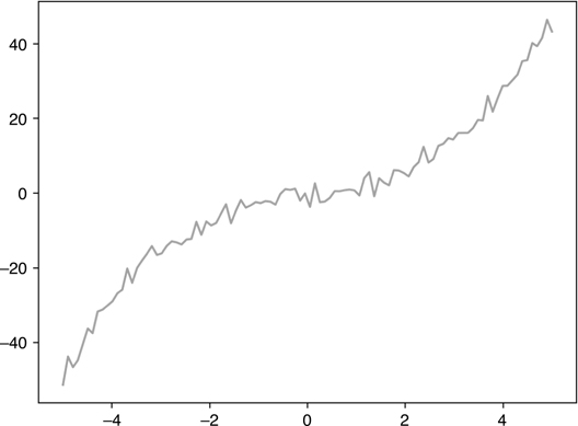
FIGURE 2.6 Datasets with potential linear regression, showing the output generated by the code in Listing 2.21
Now that you have seen an assortment of line graphs and scatterplots, let’s delve into linear regression, which is the topic of the next section.