
Assembling Data
We have previously discussed how to perform operations with a single table. But what if you need data from two or more tables? In this section, we will assemble data in multiple tables using joins and unions.
Connecting Tables Using JOIN
In the previous chapter, we discussed how to query data from a table. However, most of the time, the data you are interested in is spread across multiple tables. Fortunately, SQL has methods for bringing related tables together using the JOIN keyword.
To illustrate, let's take a look at two tables in our database—dealerships and salespeople.
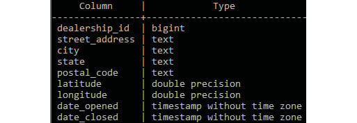
Figure 2.1: Dealerships table structure

Figure 2.2: Salespeople table structure
In the salespeople table, we observe that we have a column called dealership_id. This dealership_id column is a direct reference to the dealership_id column in the dealerships table. When table A has a column that references the primary key of table B, the column is said to be a foreign key to table A. In this case, the dealership_id column in salespeople is a foreign key to the dealerships table.
Note
Foreign keys can also be added as a column constraint to a table in order to improve the integrity of the data by making sure that the foreign key never contains a value that cannot be found in the referenced table. This data property is known as referential integrity. Adding foreign key constraints can also help to improve performance in some databases. Foreign key constraints are not used in most analytical databases and are beyond the scope of this book. You can learn more about foreign key constraints in the PostgreSQL documentation at https://www.postgresql.org/docs/9.4/tutorial-fk.html.
As these two tables are related, you can perform some interesting analyses with them. For instance, you may be interested in determining which salespeople work at a dealership in California. One way of retrieving this information is to first query which dealerships are located in California. You can do this using the following query:
SELECT
  *
FROM
  dealerships
WHERE
  state='CA';
This query should give you the following results:

Figure 2.3: Dealerships in California
Now that you know that the only two dealerships in California have the IDs of 2 and 5, respectively, you can then query the salespeople table as follows:
SELECT
  *
FROM
  salespeople
WHERE
  dealership_id in (2, 5)
ORDER BY
  1;
The following is the output of the code:
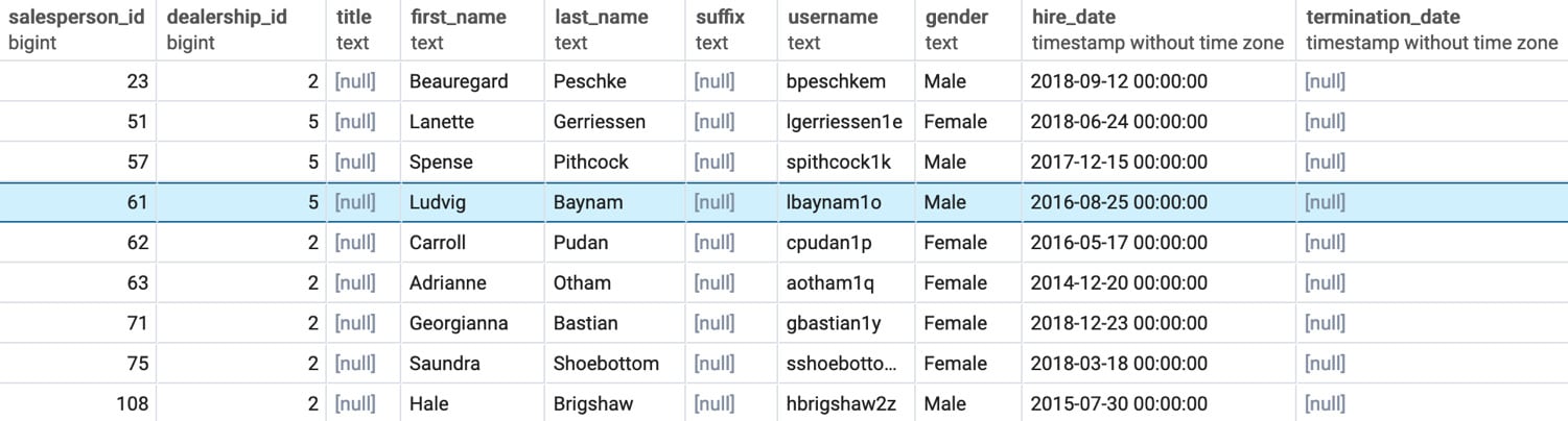
Figure 2.4: Salespeople in California
While this method gives you the results you want, it is tedious to perform two queries in order to get these results. What would make this query easier would be to somehow add the information from the dealerships table to the salespeople table and then filter for users in California. SQL provides such a tool with the JOIN clause. The JOIN clause is a SQL clause that allows a user to join one or more tables together based on distinct conditions.
Types of Joins
In this chapter, we will discuss three fundamental joins, which are illustrated in the following figure, that is, inner joins, outer joins, and cross join:
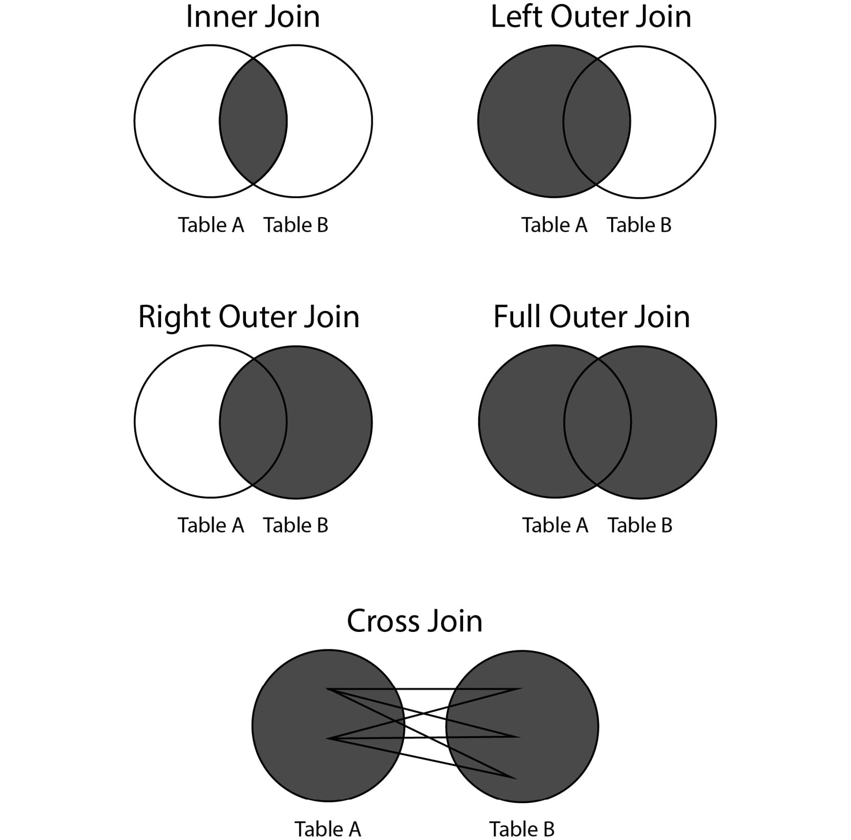
Figure 2.5: Major types of joins
Inner Joins
An inner join connects rows in different tables together, based on a condition known as the join predicate. In many cases, the join predicate is a logical condition of equality. Each row in the first table is compared against every other row in the second table. For row combinations that meet the inner join predicate, that row is returned in the query. Otherwise, the row combination is discarded.
Inner joins are usually written in the following form:
SELECT {columns}
FROM {table1}
INNER JOIN {table2} ON {table1}.{common_key_1}={table2}.{common_key_2};
Here, {columns} is the columns you want to get from the joined table, {table1} is the first table, {table2} is the second table, {common_key_1} is the column in {table1} you want to join on, and {common_key_2} is the column in {table2} to join on.
Now, let's go back to the two tables we discussed previously—dealerships and salespeople. As mentioned earlier, it would be good if we could append the information from the dealerships table to the salespeople table in order to know which state each dealer works in. For the time being, let's assume that all the salespeople IDs have a valid dealership_id value.
Note
At this point in the book, you have not learned the necessary skills to verify that every dealership ID is valid in the salespeople table, and so we assume it. However, in real-world scenarios, it will be important for you to validate these things on your own. Generally speaking, there are very few datasets and systems that guarantee clean data.
We can join the two tables using an equals condition in the join predicate, as follows:
SELECT
  *
FROM
  salespeople
INNER JOIN
  dealerships
  ON salespeople.dealership_id = dealerships.dealership_id
ORDER BY
  1;
This query will produce the following output:
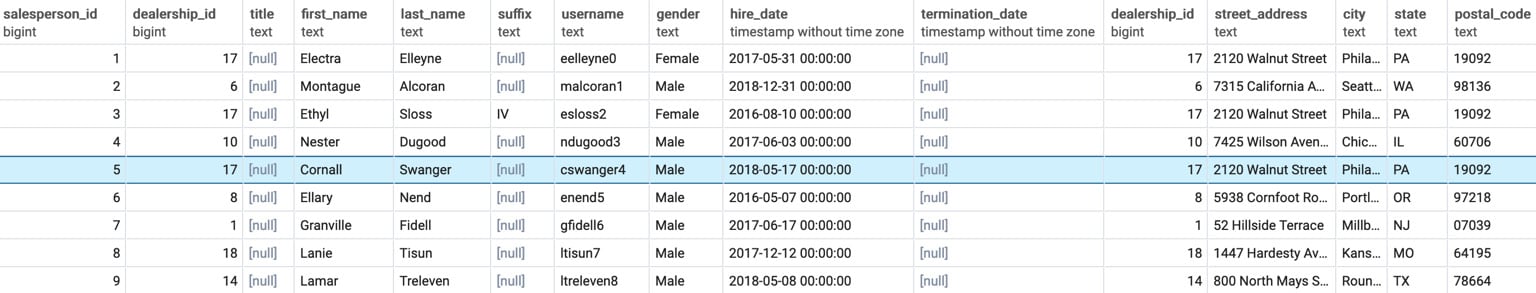
Figure 2.6: The salespeople table joined to the dealerships table
As you can see in the preceding output, the table is the result of joining the salespeople table to the dealerships table. Note that the first table listed in the query, salespeople, is on the left-hand side of the result, while the dealerships table is on the right-hand side. This is important to understand for the next section, on outer joins.
More specifically, dealership_id in the salespeople table matches dealership_id in the dealerships table. This shows how the join predicate is met. By running this join query, we have effectively created a new "super dataset" consisting of the two tables merged together where the two dealership_id columns are equal.
We can now query this "super dataset" the same way we would query one large table using the clauses and keywords from Chapter 1, Introduction to SQL for Analytics. For example, going back to our multi-query issue to determine which sales query works in California, we can now address it with one easy query:
SELECT
  *
FROM
  salespeople
INNER JOIN
  dealerships
  ON salespeople.dealership_id = dealerships.dealership_id
WHERE
  dealerships.state = 'CA'
ORDER BY
  1;
This gives us the following output:
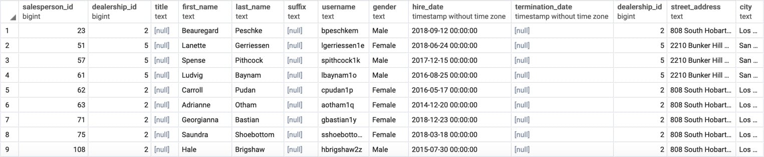
Figure 2.7: Salespeople in California with one query
You will observe that the output in Figure 2.2 and Figure 2.5 is nearly identical, with the exception being that the table in Figure 2.5 has the dealerships data appended as well. If we want to retrieve only the salespeople table portion of this, we can select the salespeople columns using the following star syntax:
SELECT
  salespeople.*
FROM
  salespeople
INNER JOIN
  dealerships
  ON dealerships.dealership_id = salespeople.dealership_id
WHERE
  dealerships.state = 'CA'
ORDER BY
  1;
There is one other shortcut that can help when writing statements with several join clauses: you can alias table names so that you do not have to type out the entire name of the table every time. Simply write the name of the alias after the first mention of the table after the join clause, and you can save a decent amount of typing. For instance, for the last preceding query, if we wanted to alias salespeople with s and dealerships with d, you could write the following statement:
SELECT
  s.*
FROM
  salespeople s
INNER JOIN
  dealerships d
  ON d.dealership_id = s.dealership_id
WHERE
  d.state = 'CA'
ORDER BY
  1;
Alternatively, you could also put the AS keyword between the table name and alias to make the alias more explicit:
SELECT
  s.*
FROM
  salespeople AS s
INNER JOIN
  dealerships AS d
  ON d.dealership_id = s.dealership_id
WHERE
  d.state = 'CA'
ORDER BY
  1;
Now that we have cleared up the basics of inner joins, we will discuss outer joins.
Outer Joins
As discussed, inner joins will only return rows from the two tables, and only if the join predicate is met for both rows. Otherwise, no rows from either table are returned. Sometimes, however, we want to return all rows from one of the tables regardless of join predicate meeting. In this case, the join predicate is not met; the row for the second table will be returned as NULL. These joins, where at least one table will be represented in every row after the join operation, are known as outer joins.
Outer joins can be classified into three categories: left outer joins, right outer joins, and full outer joins.
Left outer joins are where the left table (that is, the table mentioned first in a join clause) will have every row returned. If a row from the other table is not found, a row of NULL is returned. Left outer joins are performed by using the LEFT OUTER JOIN keywords, followed by a join predicate. This can also be written in short as LEFT JOIN.
To show how left outer joins work, let's examine two tables: the customers tables and the emails table. For the time being, assume that not every customer has been sent an email, and we want to mail all customers who have not received an email. We can use a left outer join to make that happen since the left side of the join is the customers table. To help manage output, we will only limit it to the first 1,000 rows. The following code snippet is utilized:
SELECT
  *
FROM
  customers c
LEFT OUTER JOIN
  emails e ON e.customer_id=c.customer_id
ORDER BY
  c.customer_id
LIMIT
  1000;
The following is the output of the preceding code:
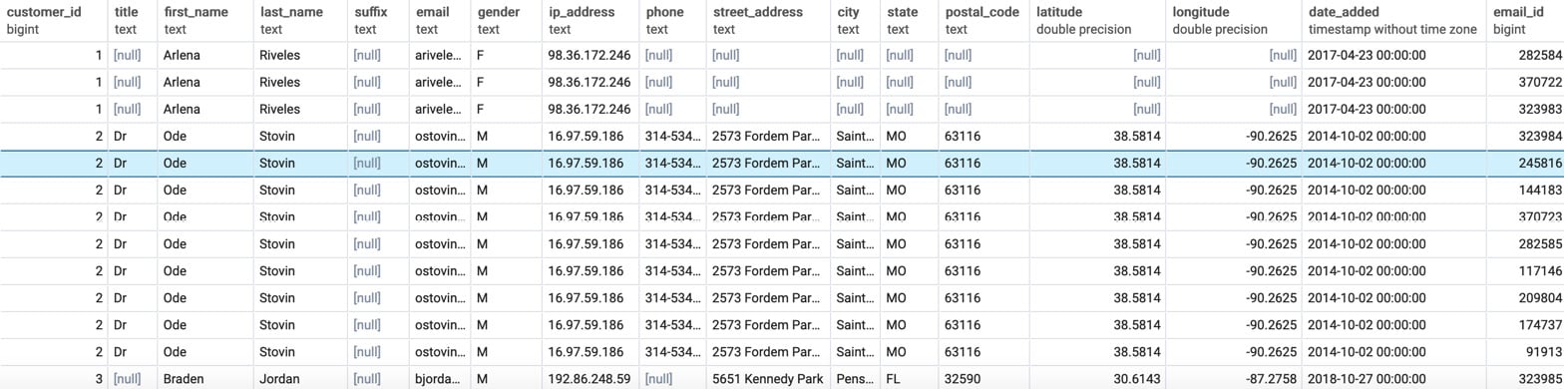
Figure 2.8: Customers left-joined to emails
When you look at the output of the query, you should see that entries from the customers table are present. However, for some of the rows, such as for customer row 27, which can be seen in Figure 2.7, the columns belonging to the emails table are completely full of NULL values. This arrangement explains how the outer join is different from the inner join. If the inner join was used, the customer_id column would not be blank.
This query, however, is still useful because we can now use it to find people who have never received an email. Because those customers who were never sent an email have a null customer_id column in the emails table, we can find all of these customers by checking the customer_id column in the emails table, as follows:
SELECT
    c.customer_id,
    c.title,
    c.first_name,
    c.last_name,
    c.suffix,
    c.email,
    c.gender,
    c.ip_address,
    c.phone,
    c.street_address,
    c.city,
    c.state,
    c.postal_code,
    c.latitude,
    c.longitude,
    c.date_added,
    e.email_id,
    e.email_subject,
    e.opened,
    e.clicked,
    e.bounced,
    e.sent_date,
    e.opened_date,
    e.clicked_date
FROM
  customers c
LEFT OUTER JOIN
  emails e ON c.customer_id = e.customer_id
WHERE
  e.customer_id IS NULL
ORDER BY
  c.customer_id
LIMIT
  1000;
The following is the output of the query:
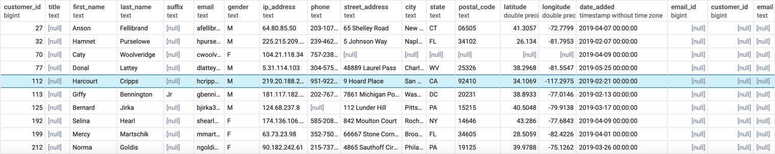
Figure 2.9: Customers with no emails sent
As you can see, all entries are blank in the customer_id column of emails table, indicating that they have not received any emails. We could simply grab the emails from this join to get all of the customers who have not received an email.
A right outer join is very similar to a left join, except the table on the "right" (the second listed table) will now have every row show up, and the "left" table will have NULL values if the join condition is not met. To illustrate, let's "flip" the last query by right-joining the emails table to the customers table with the following query:
SELECT c.customer_id,
    c.title,
    c.first_name,
    c.last_name,
    c.suffix,
    c.email,
    c.gender,
    c.ip_address,
    c.phone,
    c.street_address,
    c.city,
    c.state,
    c.postal_code,
    c.latitude,
    c.longitude,
    c.date_added,
    e.email_id,
    e.email_subject,
    e.opened,
    e.clicked,
    e.bounced,
    e.sent_date,
    e.opened_date,
    e.clicked_date
FROM
  emails e
RIGHT OUTER JOIN
  customers c ON e.customer_id=c.customer_id
ORDER BY
  c.customer_id
LIMIT
  1000;
When you run this query, you will get something similar to the following result:
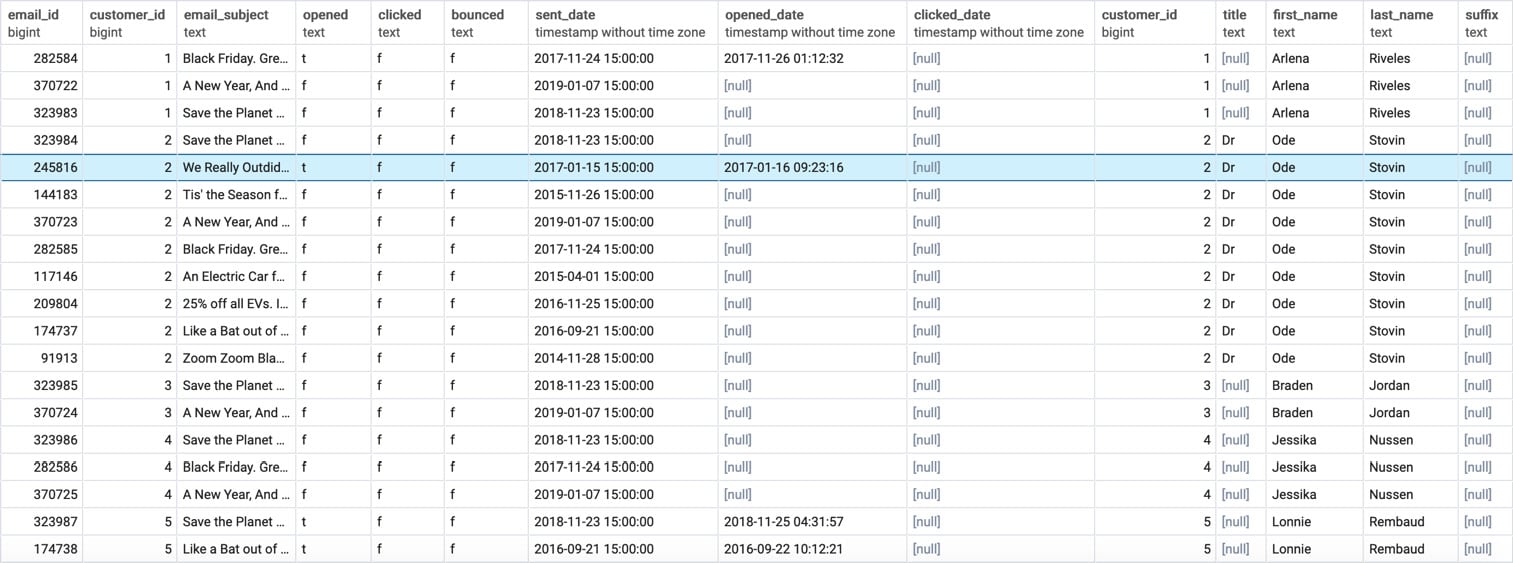
Figure 2.10: Emails right-joined to the customers table
Notice that this output is similar to what was produced in Figure 2.7, except that the data from the emails table is now on the left-hand side, and the data from the customers table is on the right-hand side. Once again, customer_id 27 has NULL for the email. This shows the symmetry between a right join and a left join.
Finally, there is the full outer join. The full outer join will return all rows from the left and right tables, regardless of whether the join predicate is matched. For rows where the join predicate is met, the two rows are combined in a group. For rows where they are not met, the row has NULL filled in. The full outer join is invoked by using the FULL OUTER JOIN clause, followed by a join predicate. Here is the syntax of this join:
SELECT
  *
FROM
  emails e
FULL OUTER JOIN
  customers c
  ON e.customer_id=c.customer_id;
The following is the output of the code:
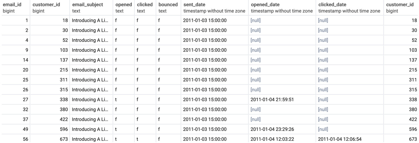
Figure 2.11: Emails are full outer joined to the customers table
In this section, we learned how to implement three different outer joins. In the next section, we will work with the cross join.
Cross Joins
The final type of join we will discuss in this book is the cross join. The cross join is also referred to as the Cartesian product; it returns every possible combination of rows from the "left" table and the "right" table. It can be invoked using a CROSS JOIN clause, followed by the name of the other table. For instance, let's take the example of the products table.
Let's say we wanted to know every possible combination of two products that you could create from a given set of products (such as the one found in the products table) in order to create a 2-month giveaway for marketing purposes. We can use a cross join to get the answer to the question using the following query:
SELECT
  p.product_id, p.model,
  c.city, c.number_of_customers
FROM
  products p1
CROSS JOIN
  products p2;
The output of this query is as follows:
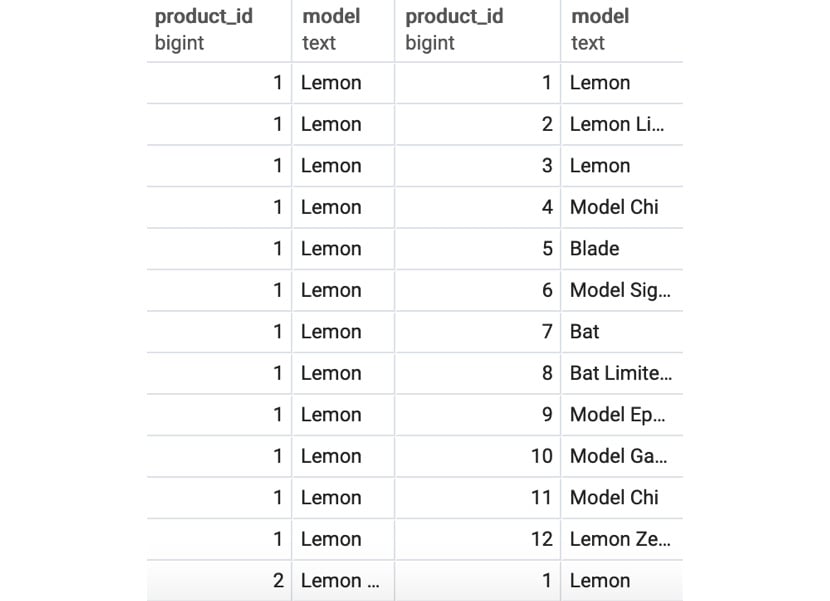
Figure 2.12: The cross join of a product to itself
You will observe that, in this particular case, we have joined every value of every field in one table to every value of every field in another table. The result of the query has 240 rows, which is the equivalent of multiplying the 12 products by the 20 top cities (12 * 20). We can also see that there is no need for a join predicate; indeed, a cross join can simply be thought of as just an outer join with no conditions for joining.
In general, cross joins are not used in practice, and can also be very dangerous if you are not careful. Cross joining two large tables together can lead to the origination of hundreds of billions of rows, which can stall and crash a database. Take care when using them.
Note
To learn more about joins, please refer to the PostgreSQL documentation at https://www.postgresql.org/docs/9.1/queries-table-expressions.html.
So far, we have covered the basics of using joins to bring tables together. We will now talk about methods for joining queries together in a dataset.
Exercise 2.01: Using Joins to Analyze a Sales Dealership
In this exercise, we will use joins to bring related tables together. The head of sales at your company would like a list of all customers who bought a car. We need to create a query that will return all customer IDs, first names, last names, and valid phone numbers of customers who purchased a car.
Note
For all exercises in this book, we will be using pgAdmin 4. All the code files for the exercises and the activity in this chapter are also available on GitHub at https://packt.live/3hf91Ch.
To solve this problem, perform the following steps:
- Open your favorite SQL client and connect to the
sqldadatabase. - Use an inner join to bring the tables
salesandcustomerstogether, which returns data for the following: customer IDs, first names, last names, and valid phone numbers:SELECT c.customer_id, c.first_name, c.last_name, c.phone FROM sales s INNER JOIN customers c ON c.customer_id=s.customer_id INNER JOIN products p ON p.product_id=s.product_id WHERE p.product_type='automobile' AND c.phone IS NOT NULL;
You should get an output similar to the following:
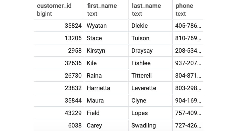
Figure 2.13: Customers who bought a car
We can see that after running the query, we were able to join the data from the sales and customers tables and obtain a list of customers who bought a car.
Note
To access the source code for this specific section, please refer to https://packt.live/2XTzNbr.
In this exercise, using joins, we were able to bring together related data easily and efficiently.
Subqueries
So far, we have been pulling data from tables. However, you may have observed that all SELECT queries produce tables as an output. Knowing this, you may wonder whether there is some way to use the tables produced by the SELECT queries instead of referencing an existing table in your database. The answer is yes. You can simply take a query, insert it between a pair of parentheses, and give it an alias. For example, if we wanted to find all the salespeople working in California and get the results the same as in Figure 2.5, we could have written the query using the following alternative:
SELECT
  *
FROM
  salespeople
INNER JOIN (
  SELECT
    *
  FROM
     dealerships
  WHERE
    dealerships.state = 'CA'
  ) d
ON d.dealership_id = salespeople.dealership_id
ORDER BY
  1;
Here, instead of joining the two tables and filtering for rows with the state equal to 'CA', we first find the dealerships where the state equals 'CA', and then inner join the rows in that query to salespeople.
If a query only has one column, you can use a subquery with the IN keyword in a WHERE clause. For example, another way to extract the details from the salespeople table using the dealership ID for the state of California would be as follows:
SELECT
  *
FROM
  salespeople
WHERE dealership_id IN (
  SELECT dealership_id FROM dealerships
  WHERE dealerships.state = 'CA'
  )
ORDER BY
  1;
As all of these examples show, it's quite easy to write the same query using multiple techniques. In the next section, we will talk about unions.
Unions
So far, we have been talking about how to join data horizontally. That is, with joins, new columns are effectively added horizontally. However, we may be interested in putting multiple queries together vertically, that is, by keeping the same number of columns but adding multiple rows. An example may help to clarify this.
Say that you wanted to visualize the addresses of dealerships and customers using Google Maps. To do this, you would need both the addresses of customers and dealerships. You could build a query with all customer addresses as follows:
SELECT
  street_address, city, state, postal_code
FROM
  customers
WHERE
  street_address IS NOT NULL;
You could also retrieve dealership addresses with the following query:
SELECT
  street_address, city, state, postal_code
FROM
  dealerships
WHERE
  street_address IS NOT NULL;
However, it would be nice if we could assemble the two queries together into one list with one query. This is where the UNION keyword comes into play. Using the two previous queries, we could create the following query:
(
SELECT
  street_address, city, state, postal_code
FROM
  customers
WHERE
  street_address IS NOT NULL
)
UNION
(
SELECT
  street_address, city, state, postal_code
FROM
  dealerships
WHERE
  street_address IS NOT NULL
)
ORDER BY
  1;
This produces the following output:
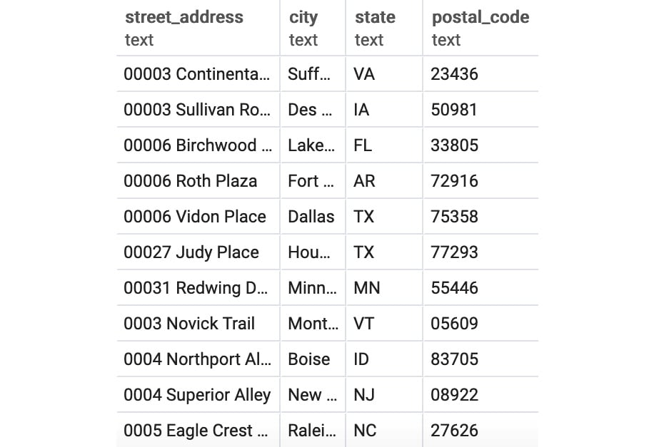
Figure 2.14: Union of addresses
There are some caveats to using UNION. First, UNION requires that the subqueries there have the same name columns and the same data types for the column. If it does not, the query will not run. Second, UNION technically may not return all the rows from its subqueries. UNION, by default, removes all duplicate rows in the output. If you want to retain the duplicate rows, it is preferable to use the UNION ALL keyword. In the next exercise, we will implement union operations.
Exercise 2.02: Generating an Elite Customer Party Guest List Using UNION
In this exercise, we will assemble two queries using unions. In order to help build up marketing awareness for the new Model Chi, the marketing team would like to throw a party for some of ZoomZoom's wealthiest customers in Los Angeles, CA. To help facilitate the party, they would like you to make a guest list with ZoomZoom customers who live in Los Angeles, CA, as well as salespeople who work at the ZoomZoom dealership in Los Angeles, CA. The guest list should include first and last names and whether the guest is a customer or an employee.
To solve this problem, execute the following:
- Open your favorite SQL client and connect to the
sqldadatabase. - Write a query that will make a list of ZoomZoom customers and company employees who live in Los Angeles, CA. The guest list should contain first and last names and whether the guest is a customer or an employee:
(
SELECT
  first_name, last_name, 'Customer' as guest_type
FROM
  customers
WHERE
  city='Los Angeles'
  AND state='CA'
)
UNION
(
SELECT
  first_name, last_name,
  'Employee' as guest_type
FROM
  salespeople s
INNER JOIN
  dealerships d ON d.dealership_id=s.dealership_id
WHERE
  d.city='Los Angeles'
  AND d.state='CA'
)
You should get the following output:
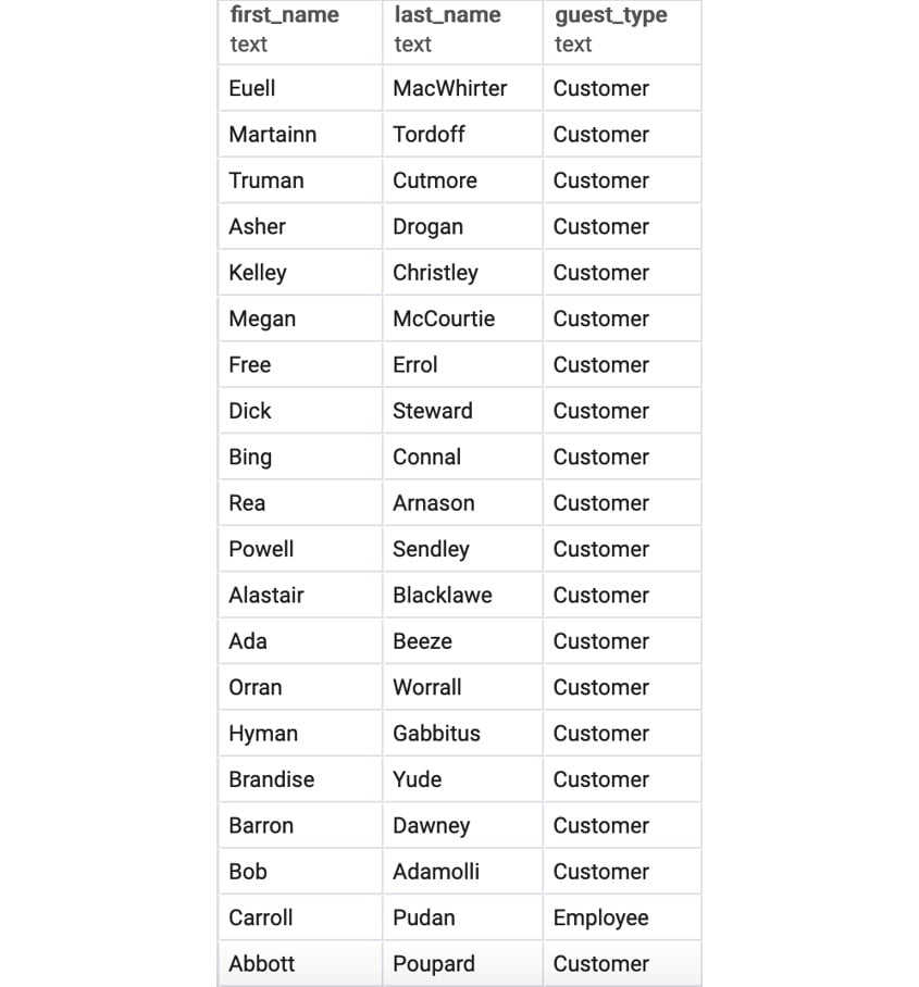
Figure 2.15: Customer and employee guest list in Los Angeles, CA
We can see the guest list of customers and employees from Los Angeles, CA, after running the UNION query.
Note
To access the source code for this specific section, please refer to https://packt.live/3ffQq79.
In the exercise, we used the UNION keyword to combine rows from different queries effortlessly. In the next section, we will learn about common table expressions.
Common Table Expressions
Common table expressions are, in a certain sense, just a different version of subqueries. Common table expressions establish temporary tables by using the WITH clause. To understand this clause better, let's take a look at the following query, which we've used before to find California-based salespeople:
SELECT
  *
FROM
  salespeople
INNER JOIN (
  SELECT
    *
  FROM
    dealerships
  WHERE
    dealerships.state = 'CA'
  ) d
ON d.dealership_id = salespeople.dealership_id
ORDER BY
  1;
This could be written using common table expressions as follows:
WITH d as (
  SELECT
    *
  FROM
    dealerships
  WHERE
    dealerships.state = 'CA'
  )
SELECT
  *
FROM
  salespeople
INNER JOIN
  d ON d.dealership_id = salespeople.dealership_id
ORDER BY
  1;
The one advantage of common table expressions is that they are recursive. Recursive common table expressions can reference themselves. Because of this feature, we can use them to solve problems that other queries cannot. However, recursive common table expressions are beyond the scope of this book.
Now that we know several ways to join data together across a database, we will look at how to transform the data from these outputs.