Performing multivariate imputation by chained equations

Multivariate imputation methods, as opposed to univariate imputation, use the entire set of variables to estimate the missing values. In other words, the missing values of a variable are modeled based on the other variables in the dataset. Multivariate imputation by chained equations (MICE) is a multiple imputation technique that models each variable with missing values as a function of the remaining variables and uses that estimate for imputation. MICE has the following basic steps:

1. A simple univariate imputation is performed for every variable with missing data, for example, median imputation.
2. One specific variable is selected, say, var_1, and the missing values are set back to missing.
3. A model that's used to predict var_1 is built based on the remaining variables in the dataset.
4. The missing values of var_1 are replaced with the new estimates.
5. Repeat step 2 to step 4 for each of the remaining variables.

Once all the variables have been modeled based on the rest, a cycle of imputation is concluded. Step 2 to step 4 are performed multiple times, typically 10 times, and the imputation values after each round are retained. The idea is that, by the end of the cycles, the distribution of the imputation parameters should have converged.

Each variable with missing data can be modeled based on the remaining variable by using multiple approaches, for example, linear regression, Bayes, decision trees, k-nearest neighbors, and random forests.

In this recipe, we will implement MICE using scikit-learn.

Getting ready

To learn more about MICE, take a look at the following links:

• A multivariate technique for multiplying imputing missing values using a sequence of regression models: http://citeseerx.ist.psu.edu/viewdoc/download?doi=10.1.1.405.4540&rep=rep1&type=pdf

• Multiple Imputation by Chained Equations: What is it and how does it work?: https://www.ncbi.nlm.nih.gov/pmc/articles/PMC3074241/

• Scikit-learn: https://scikit-learn.org/stable/modules/impute.html

In this recipe, we will perform MICE imputation using IterativeImputer() from scikit-learn: https://scikit-learn.org/stable/modules/generated/sklearn.impute.IterativeImputer.html#sklearn.impute.IterativeImputer.

To follow along with this recipe, prepare the Credit Approval Data Set, as specified in the Technical requirements section of this chapter.

For this recipe, make sure you are using scikit-learn version 0.21.2 or above.

How to do it...

To complete this recipe, let's import the required libraries and load the data:

1.  Let's import the required Python libraries and classes:

import pandas as pd
from sklearn.model_selection import train_test_split
from sklearn.linear_model import BayesianRidge
from sklearn.experimental import enable_iterative_imputer
from sklearn.impute import IterativeImputer

2. Let's load the dataset with some numerical variables:

variables = ['A2','A3','A8', 'A11', 'A14', 'A15', 'A16']
data = pd.read_csv('creditApprovalUCI.csv', usecols=variables)

The models that will be used to estimate missing values should be built on the train data and used to impute values in the train, test, and future data:

3. Let's divide the data into train and test sets:

X_train, X_test, y_train, y_test = train_test_split(
    data.drop('A16', axis=1),data['A16' ], test_size=0.3, 
    random_state=0)

4. Let's create a MICE imputer using Bayes regression as an estimator, specifying the number of iteration cycles and setting random_state for reproducibility:

imputer = IterativeImputer(estimator = BayesianRidge(), max_iter=10, random_state=0)

IterativeImputer() contains other useful arguments. For example, we can specify the first imputation strategy using the initial_strategy parameter and specify how we want to cycle over the variables either randomly, or from the one with the fewest missing values to the one with the most.

5. Let's fit IterativeImputer() to the train set so that it trains the estimators to predict the missing values in each variable:

imputer.fit(X_train)

6. Finally, let's fill in missing values in both train and test set:

X_train = imputer.transform(X_train)
X_test = imputer.transform(X_test)

Remember that scikit-learn returns NumPy arrays and not dataframes.

How it works...

In this recipe, we performed MICE using IterativeImputer() from scikit-learn. First, we loaded data using pandas read_csv() and separated it into train and test sets using scikit-learn's train_test_split(). Next, we created a multivariate imputation object using the IterativeImputer() from scikit-learn. We specified that we wanted to estimate missing values using Bayes regression and that we wanted to carry out 10 rounds of imputation over the entire dataset. We fitted IterativeImputer() to the train set so that each variable was modeled based on the remaining variables in the dataset. Next, we transformed the train and test sets with the transform() method in order to replace missing data with their estimates.

There's more...

Using IterativeImputer() from scikit-learn, we can model variables using multiple algorithms, such as Bayes, k-nearest neighbors, decision trees, and random forests. Perform the following steps to do so:

1. Import the required Python libraries and classes:

import pandas as pd
import matplotlib.pyplot as plt
from sklearn.model_selection import train_test_split
from sklearn.linear_model import BayesianRidge
from sklearn.tree import DecisionTreeRegressor
from sklearn.ensemble import ExtraTreesRegressor
from sklearn.neighbors import KNeighborsRegressor

2. Load the data and separate it into train and test sets:

variables = ['A2','A3','A8', 'A11', 'A14', 'A15', 'A16']
data = pd.read_csv('creditApprovalUCI.csv', usecols=variables)

X_train, X_test, y_train, y_test = train_test_split(
    data.drop('A16', axis=1), data['A16'], test_size=0.3, 
        random_state=0)

3. Build MICE imputers using different modeling strategies:

imputer_bayes = IterativeImputer(
    estimator=BayesianRidge(),
    max_iter=10,
    random_state=0)

imputer_knn = IterativeImputer(
    estimator=KNeighborsRegressor(n_neighbors=5),
    max_iter=10,
    random_state=0)

imputer_nonLin = IterativeImputer(
    estimator=DecisionTreeRegressor(
        max_features='sqrt', random_state=0),
    max_iter=10,
    random_state=0)

imputer_missForest = IterativeImputer(
    estimator=ExtraTreesRegressor(
        n_estimators=10, random_state=0),

    max_iter=10,
    random_state=0)

Note how, in the preceding code block, we create four different MICE imputers, each with a different machine learning algorithm which will be used to model every variable based on the remaining variables in the dataset.

4. Fit the MICE imputers to the train set:

imputer_bayes.fit(X_train)
imputer_knn.fit(X_train)
imputer_nonLin.fit(X_train)
imputer_missForest.fit(X_train)

5. Impute missing values in the train set:

X_train_bayes = imputer_bayes.transform(X_train)
X_train_knn = imputer_knn.transform(X_train)
X_train_nonLin = imputer_nonLin.transform(X_train)
X_train_missForest = imputer_missForest.transform(X_train)

Remember that scikit-learn transformers return NumPy arrays.

6. Convert the NumPy arrays into dataframes:

predictors = [var for var in variables if var !='A16']
X_train_bayes = pd.DataFrame(X_train_bayes, columns = predictors)
X_train_knn = pd.DataFrame(X_train_knn, columns = predictors)
X_train_nonLin = pd.DataFrame(X_train_nonLin, columns = predictors)
X_train_missForest = pd.DataFrame(X_train_missForest, columns = predictors)

7. Plot and compare the results:

fig = plt.figure()
ax = fig.add_subplot(111)

X_train['A3'].plot(kind='kde', ax=ax, color='blue')
X_train_bayes['A3'].plot(kind='kde', ax=ax, color='green')
X_train_knn['A3'].plot(kind='kde', ax=ax, color='red')
X_train_nonLin['A3'].plot(kind='kde', ax=ax, color='black')
X_train_missForest['A3'].plot(kind='kde', ax=ax, color='orange')

# add legends
lines, labels = ax.get_legend_handles_labels()
labels = ['A3 original', 'A3 bayes', 'A3 knn', 'A3 Trees', 'A3 missForest']
ax.legend(lines, labels, loc='best')
plt.show()

The output of the preceding code is as follows:

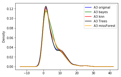
In the preceding plot, we can see that the different algorithms return slightly different distributions of the original variable.