Preparing and testing the train script in R
In this recipe, we will write a custom train script in R that allows us to inspect the input and configuration parameters set by Amazon SageMaker during the training process. The following diagram shows the train script inside the custom container, which makes use of the hyperparameters, input data, and configuration specified in the Estimator instance using the SageMaker Python SDK and the reticulate package:
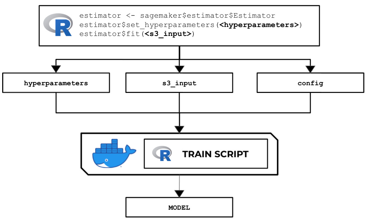
Figure 2.79 – The R train script inside the custom container makes use of the input parameters, configuration, and data to train and output a model
There are several options when running a training job – use a built-in algorithm, use a custom train script and custom Docker images, or use a custom train script and prebuilt Docker images. In this recipe, we will focus on the second option, where we will prepare and test a bare minimum training script in R that builds a linear model for a specific regression problem.
Once we have finished working on this recipe, we will have a better understanding of how SageMaker works behind the scenes. We will see where and how to load and use the configuration and arguments we have specified in the SageMaker Python SDK Estimator instance.
Important note
Later on, you will notice a few similarities between the Python and R recipes in this chapter. What is critical here is noticing and identifying both major and subtle differences in certain parts of the Python and R recipes. For example, when working with the serve script in this chapter, we will be dealing with two files in R (api.r and serve) instead of one in Python (serve). As we will see in the other recipes of this book, working on the R recipes will help us have a better understanding of the internals of SageMaker's capabilities, as there is a big chance that we will have to prepare custom solutions to solve certain requirements. As we get exposed to more machine learning requirements, we will find that there are packages in R for machine learning without direct counterparts in Python. That said, we must be familiar with how to get custom R algorithm code working in SageMaker. Stay tuned for more!
Getting ready
Make sure you have completed the Setting up the Python and R experimentation environments recipe.
How to do it...
The first set of steps in this recipe focus on preparing the train script. Let's get started:
- Inside the
ml-rdirectory, double-click thetrainfile to open it inside the Editor pane:
Figure 2.80 – Empty ml-r/train file
Here, we have an empty train file. In the lower-right-hand corner of the Editor pane, you can change the syntax highlight settings to R.
- Add the following lines of code to start the
trainscript in order to import the required packages and libraries:#!/usr/bin/Rscript library("rjson") - Define the
prepare_paths()function, which we will use to initialize thePATHSvariable. This will help us manage the paths of the primary files and directories used in the script:prepare_paths <- function() { keys <- c('hyperparameters', 'input', 'data', 'model') values <- c('input/config/hyperparameters.json', 'input/config/inputdataconfig.json', 'input/data/', 'model/') paths <- as.list(values) names(paths) <- keys return(paths); } PATHS <- prepare_paths()This function allows us to initialize the
PATHSvariable with a dictionary-like data structure where we can get the absolute paths of the required file. - Next, define the
get_path()function, which makes use of thePATHSvariable from the previous step:get_path <- function(key) { output <- paste('/opt/ml/', PATHS[[key]], sep="") return(output); }When referring to the location of a specific file, such as
hyperparameters.json, we will useget_path('hyperparameters')instead of the absolute path. - Next, add the following lines of code just after the
get_path()function definition from the previous step. These functions will be used to load and print the contents of the JSON files we will work with later:load_json <- function(target_file) { result <- fromJSON(file = target_file) } print_json <- function(target_json) { print(target_json) } - After that, define the
inspect_hyperparameters()andlist_dir_contents()functions after theprint_json()function definition:inspect_hyperparameters <- function() { hyperparameters_json_path <- get_path( 'hyperparameters' ) print(hyperparameters_json_path) hyperparameters <- load_json( hyperparameters_json_path ) print(hyperparameters) } list_dir_contents <- function(target_path) { print(list.files(target_path)) }The
inspect_hyperparameters()function inspects the contents of thehyperparameters.jsonfile inside the/opt/ml/input/configdirectory. Thelist_dir_contents()function, on the other hand, displays the contents of a target directory. - Define the
inspect_input()function. It will help us inspect the contents ofinputdataconfig.jsoninside the/opt/ml/input/configdirectory:inspect_input <- function() { input_config_json_path <- get_path('input') print(input_config_json_path) input_config <- load_json( input_config_json_path ) print_json(input_config) for (key in names(input_config)) { print(key) input_data_dir <- paste(get_path('data'), key, '/', sep="") print(input_data_dir) list_dir_contents(input_data_dir) } }This will be used to list the contents of the training input directory inside the
main()function later. - Define the
load_training_data()function:load_training_data <- function(input_data_dir) { print('[load_training_data]') files <- list_dir_contents(input_data_dir) training_data_path <- paste0( input_data_dir, files[[1]]) print(training_data_path) df <- read.csv(training_data_path, header=FALSE) colnames(df) <- c("y","X") print(df) return(df) }This function can be divided into two parts – preparing the specific path pointing to the CSV file containing the training data and reading the contents of the CSV file using the
read.csv()function. The return value of this function is an R DataFrame (a two-dimensional table-like structure). - Next, define the
get_input_data_dir()function:get_input_data_dir <- function() { print('[get_input_data_dir]') key <- 'train' input_data_dir <- paste0( get_path('data'), key, '/') return(input_data_dir) } - After that, define the
train_model()function:train_model <- function(data) { model <- lm(y ~ X, data=data) print(summary(model)) return(model) }This function makes use of the
lm()function to fit and prepare linear models, which can then be used for regression tasks. It accepts a formula such asy ~ Xas the first parameter value and the training dataset as the second parameter value.Note
Formulas in R involve a tilde symbol (
~) and one or more independent variables at the right of the tilde (~), such asX1 + X2 + X3. In the example in this recipe, we only have one variable on the right-hand side of the tilde (~), meaning that we will only have a single predictor variable for this model. On the left-hand side of the tilde (~) is the dependent variable that we are trying to predict using the predictor variable(s). That said, they ~ Xformula simply expresses a relationship between the predictor variable,X, and theyvariable we are trying to predict. Since we are dealing with the same dataset as we did for the recipes in Chapter 1, Getting Started with Machine Learning Using Amazon SageMaker, theyvariable here maps tomonthly_salary, whileXmaps tomanagement_experience_months. - Define the
save_model()function:save_model <- function(model) { print('[save_model]') filename <- paste0(get_path('model'), 'model') print(filename) saveRDS(model, file=filename) print('Model Saved!') }Here, we make use of the
saveRDS()function, which accepts an R object and writes it to a file. In this case, we will accept a trained model object and save it inside the/opt/ml/modeldirectory. - Define the
main()function, as shown here. This function triggers the functions defined in the previous steps:main <- function() { inspect_hyperparameters() inspect_input() input_data_dir = get_input_data_dir() print(input_data_dir) data <- load_training_data(input_data_dir) model <- train_model(data) save_model(model) }This
main()function can be divided into four parts – inspecting the hyperparameters and the input, loading the training data, training the model using thetrain_model()function, and saving the model using thesave_model()function. - Finally, call the
main()function at the end of the script:main()
Tip
You can access a working copy of the train file in the Machine Learning with Amazon SageMaker Cookbook GitHub repository: https://github.com/PacktPublishing/Machine-Learning-with-Amazon-SageMaker-Cookbook/blob/master/Chapter02/ml-r/train.
Now that we are done with the
trainscript, we will use the Terminal to perform the last set of steps in this recipe. The last set of steps focus on installing a few script prerequisites. - Open a new Terminal:

Figure 2.81 – New Terminal
Here, we can see how to create a new Terminal tab. We simply click the plus (+) button and then choose New Terminal.
- Check the version of R in the Terminal:
R --version
Running this line of code should return a similar set of results to what is shown here:

Figure 2.82 – Result of the R --version command in the Terminal
Here, we can see that our environment is using R version
3.4.4. - Install the
rjsonpackage:sudo R -e "install.packages('rjson',repos='https://cloud.r-project.org')"The
rjsonpackage provides the utilities for handling JSON data in R. - Use the following commands to make the
trainscript executable and then run thetrainscript:cd /home/ubuntu/environment/opt/ml-r chmod +x train ./train
Running the previous lines of code will yield results similar to what is shown here:
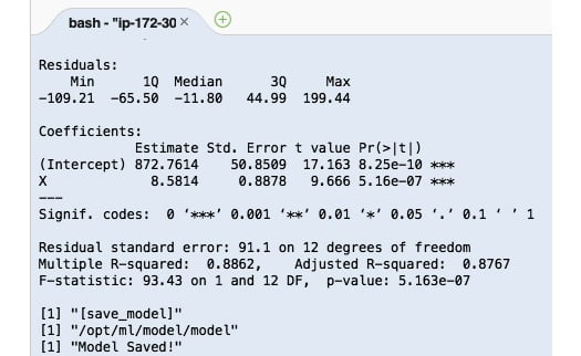
Figure 2.83 – R train script output
Here, we can see the logs that were produced by the train script. Once the train script has been successfully executed, we expect the model files to be stored inside the /opt/ml/model directory.
At this point, we have finished preparing and testing the train script. Now, let's see how this works!
How it works…
The train script in this recipe demonstrates how the input and output values are passed around between the SageMaker API and the custom container. It also performs a fairly straightforward set of steps to train a linear model using the training data provided.
When you are required to work on a more realistic example, the train script will do the following:
- Load and use a few environment variables using the
Sys.getenv()function in R. We can load environment variables set by SageMaker automatically, such asTRAINING_JOB_NAMEandTRAINING_JOB_ARN. - Load the contents of the
hyperparameters.jsonfile using thefromJSON()function. - Load the contents of the
inputdataconfig.jsonfile using thefromJSON()function. This file contains the properties of each of the input data channels, such as the file type and usage of thefileorpipemode. - Load the data file(s) inside the
/opt/ml/input/datadirectory. Take note that there's a parent directory named after the input data channel in the path before the actual files themselves. An example of this would be/opt/ml/input/data/<channel name>/<filename>. - Perform model training using the hyperparameters and training data that was loaded in the previous steps.
- Save the model inside the
/opt/ml/modeldirectory:saveRDS(model, file="/opt/ml/model/model.RDS")
- We can optionally evaluate the model using the validation data and log the results.
Now that have finished preparing the train script in R, let's quickly discuss some possible solutions we can prepare using what we learned in this recipe.
There's more…
It is important to note that we are free to use any algorithm in the train script to train our model. This level of flexibility gives us an edge once we need to work on more complex examples. Here is a quick example of what the train function may look like if the neuralnet R package is used in the train script:
train <- function(df.training_data, hidden_layers=4) {
    model <- neuralnet(
        label ~ .,
        df.training_data,
        hidden=c(hidden_layers,1),
        linear.output = FALSE,
        threshold=0.02,
        stepmax=1000000,
        act.fct = "logistic")
    return(model)
}
In this example, we allow the number of hidden layers to be set while we are configuring the Estimator object using the set_hyperparameters() function. The following example shows how to implement a train function to prepare a time series forecasting model in R:
train <- function(data) {
    model <- snaive(data)
    print(summary(model))
    return(model)
}
Here, we simply used the snaive() function from the forecast package to prepare the model. Of course, we are free to use other functions as well, such as ets() and auto.arima() from the forecast package.