Search icon CANCEL
Subscription
0
Cart icon
Your Cart (0 item)
Close icon
You have no products in your basket yet
Arrow left icon
Explore Products
Best Sellers
New Releases
Books
Events
Videos
Audiobooks
Packt Hub
Free Learning
Arrow right icon
timer SALE ENDS IN
0 Days
:
00 Hours
:
00 Minutes
:
00 Seconds
The Unsupervised Learning Workshop

The Unsupervised Learning Workshop: Get started with unsupervised learning algorithms and simplify your unorganized data to help make future predictions

Arrow left icon
Profile Icon Aaron Jones Profile Icon Christopher Kruger Profile Icon Benjamin Johnston Profile Icon Richard Brooker Profile Icon John Wesley Doyle Profile Icon Priyanjit Ghosh Profile Icon Sani Kamal Profile Icon Ashish Pratik Patil Profile Icon Philip Solomon Profile Icon Geetank Raipuria +6 more Show less
Arrow right icon
₹999.99 ₹2740.99
Full star icon Full star icon Full star icon Full star icon Half star icon 4.3 (6 Ratings)
eBook Jul 2020 550 pages 1st Edition
eBook
₹999.99 ₹2740.99
Paperback
₹3425.99
Paperback
₹3276.99
eBook + Subscription
₹1000 Monthly
eBook
₹999.99 ₹2740.99
Paperback
₹3425.99
Paperback
₹3276.99
eBook + Subscription
₹1000 Monthly

What do you get with eBook?

Product feature icon Instant access to your Digital eBook purchase
Product feature icon Download this book in EPUB and PDF formats
Product feature icon Access this title in our online reader with advanced features
Product feature icon DRM FREE - Read whenever, wherever and however you want
Product feature icon AI Assistant (beta) to help accelerate your learning
Modal Close icon
Payment Processing...
tick Completed

Billing Address

Table of content icon View table of contents Preview book icon Preview Book

The Unsupervised Learning Workshop

2. Hierarchical Clustering

Overview

In this chapter, we will implement the hierarchical clustering algorithm from scratch using common Python packages and perform agglomerative clustering. We will also compare k-means with hierarchical clustering. We will use hierarchical clustering to build stronger groupings that make more logical sense. By the end of this chapter, we will be able to use hierarchical clustering to build stronger groupings that make more logical sense.

Introduction

In this chapter, we will expand on the basic ideas that we built in Chapter 1, Introduction to Clustering, by surrounding clustering with the concept of similarity. Once again, we will be implementing forms of the Euclidean distance to capture the notion of similarity. It is important to bear in mind that the Euclidean distance just happens to be one of the most popular distance metrics; it's not the only one. Through these distance metrics, we will expand on the simple neighbor calculations that we explored in the previous chapter by introducing the concept of hierarchy. By using hierarchy to convey clustering information, we can build stronger groupings that make more logical sense. Similar to k-means, hierarchical clustering can be helpful for cases such as customer segmentation or identifying similar product types. However, there is a slight benefit in being able to explain things in a clearer fashion with hierarchical clustering. In this chapter, we will outline some cases where hierarchical clustering can be the solution you're looking for.

Clustering Refresher

Chapter 1, Introduction to Clustering, covered both the high-level concepts and in-depth details of one of the most basic clustering algorithms: k-means. While it is indeed a simple approach, do not discredit it; it will be a valuable addition to your toolkit as you continue your exploration of the unsupervised learning world. In many real-world use cases, companies experience valuable discoveries through the simplest methods, such as k-means or linear regression (for supervised learning). An example of this is evaluating a large selection of customer data – if you were to evaluate it directly in a table, it would be unlikely that you'd find anything helpful. However, even a simple clustering algorithm can identify where groups within the data are similar and dissimilar. As a refresher, let's quickly walk through what clusters are and how k-means works to find them:

Figure 2.1: The attributes that separate supervised and unsupervised problems

Figure 2.1: The attributes that separate supervised and unsupervised problems

If you were given a random collection of data without any guidance, you would probably start your exploration using basic statistics – for example, the mean, median, and mode values for each of the features. Given a dataset, choosing supervised or unsupervised learning as an approach to derive insights is dependent on the data goals that you have set for yourself. If you were to determine that one of the features was actually a label and you wanted to see how the remaining features in the dataset influence it, this would become a supervised learning problem. However, if, after initial exploration, you realized that the data you have is simply a collection of features without a target in mind (such as a collection of health metrics, purchase invoices from a web store, and so on), then you could analyze it through unsupervised methods.

A classic example of unsupervised learning is finding clusters of similar customers in a collection of invoices from a web store. Your hypothesis is that by finding out which people are the most similar, you can create more granular marketing campaigns that appeal to each cluster's interests. One way to achieve these clusters of similar users is through k-means.

The k-means Refresher

The k-means clustering works by finding "k" number of clusters in your data through certain distance calculations such as Euclidean, Manhattan, Hamming, Minkowski, and so on. "K" points (also called centroids) are randomly initialized in your data and the distance is calculated from each data point to each of the centroids. The minimum of these distances designates which cluster a data point belongs to. Once every point has been assigned to a cluster, the mean intra-cluster data point is calculated as the new centroid. This process is repeated until the newly calculated cluster centroid no longer changes position or until the maximum limit of iterations is reached.

The Organization of the Hierarchy

Both the natural and human-made world contain many examples of organizing systems into hierarchies and why, for the most part, it makes a lot of sense. A common representation that is developed from these hierarchies can be seen in tree-based data structures. Imagine that you have a parent node with any number of child nodes that can subsequently be parent nodes themselves. By organizing information into a tree structure, you can build an information-dense diagram that clearly shows how things are related to their peers and their larger abstract concepts.

An example from the natural world to help illustrate this concept can be seen in how we view the hierarchy of animals, which goes from parent classes to individual species:

Figure 2.2: The relationships of animal species in a hierarchical tree structure

Figure 2.2: The relationships of animal species in a hierarchical tree structure

In the preceding diagram, you can see an example of how relational information between varieties of animals can be easily mapped out in a way that both saves space and still transmits a large amount of information. This example can be seen as both a tree of its own (showing how cats and dogs are different, but both are domesticated animals) and as a potential piece of a larger tree that shows a breakdown of domesticated versus non-domesticated animals.

As a business-facing example, let's go back to the concept of a web store selling products. If you sold a large variety of products, then you would probably want to create a hierarchical system of navigation for your customers. By preventing all of the information in your product catalog from being presented at once, customers will only be exposed to the path down the tree that matches their interests. An example of the hierarchical system of navigation can be seen in the following diagram:

Figure 2.3: Product categories in a hierarchical tree structure

Figure 2.3: Product categories in a hierarchical tree structure

Clearly, the benefits of a hierarchical system of navigation cannot be overstated in terms of improving your customer experience. By organizing information into a hierarchical structure, you can build an intuitive structure into your data that demonstrates explicit nested relationships. If this sounds like another approach to finding clusters in your data, then you're definitely on the right track. Through the use of similar distance metrics, such as the Euclidean distance from k-means, we can develop a tree that shows the many cuts of data that allow a user to subjectively create clusters at their discretion.

Introduction to Hierarchical Clustering

So far, we have shown you that hierarchies can be excellent structures to organize information that clearly shows nested relationships among data points. While this helps us gain an understanding of the parent/child relationships between items, it can also be very handy when forming clusters. Expanding on the animal example in the previous section, imagine that you were simply presented with two features of animals: their height (measured from the tip of the nose to the end of the tail) and their weight. Using this information, you then have to recreate a hierarchical structure in order to identify which records in your dataset correspond to dogs and cats, as well as their relative subspecies.

Since you are only given animal heights and weights, you won't be able to deduce the specific names of each species. However, by analyzing the features that you have been provided with, you can develop a structure within the data that serves as an approximation of what animal species exist in your data. This perfectly sets the stage for an unsupervised learning problem that is well solved with hierarchical clustering. In the following plot, you can see the two features that we created on the left, with animal height in the left-hand column and animal weight in the right-hand column. This is then charted on a two-axis plot with the height on the X-axis and the weight on the Y-axis:

Figure 2.4: An example of a two-feature dataset comprising animal height 
and animal weight

Figure 2.4: An example of a two-feature dataset comprising animal height and animal weight

One way to approach hierarchical clustering is by starting with each data point, serving as its own cluster, and recursively joining the similar points together to form clusters – this is known as agglomerative hierarchical clustering. We will go into more detail about the different ways of approaching hierarchical clustering in the Agglomerative versus Divisive Clustering section.

In the agglomerative hierarchical clustering approach, the concept of data point similarity can be thought of in the paradigm that we saw during k-means. In k-means, we used the Euclidean distance to calculate the distance from the individual points to the centroids of the expected "k" clusters. In this approach to hierarchical clustering, we will reuse the same distance metric to determine the similarity between the records in our dataset.

Eventually, by grouping individual records from the data with their most similar records recursively, you end up building a hierarchy from the bottom up. The individual single-member clusters join into one single cluster at the top of our hierarchy.

Steps to Perform Hierarchical Clustering

To understand how agglomerative hierarchical clustering works, we can trace the path of a simple toy program as it merges to form a hierarchy:

  1. Given n sample data points, view each point as an individual "cluster" with just that one point as a member (the centroid).
  2. Calculate the pairwise Euclidean distance between the centroids of all the clusters in your data. (Here, minimum distance between clusters, maximum distance between clusters, average distance between clusters, or distance between two centroids can also be considered. In this example, we are considering the distance between two cluster centroids).
  3. Group the closest clusters/points together.
  4. Repeat Step 2 and Step 3 until you get a single cluster containing all the data in your set.
  5. Plot a dendrogram to show how your data has come together in a hierarchical structure. A dendrogram is simply a diagram that is used to represent a tree structure, showing an arrangement of clusters from top to bottom. We will go into the details of how this may be helpful in the following walkthrough.
  6. Decide what level you want to create the clusters at.

An Example Walkthrough of Hierarchical Clustering

While slightly more complex than k-means, hierarchical clustering is, in fact, quite similar to it from a logistical perspective. Here is a simple example that walks through the preceding steps in slightly more detail:

  1. Given a list of four sample data points, view each point as a centroid that is also its own cluster with the point indices from 0 to 3:
    Clusters (4): [ (1,7) ], [ (-5,9) ], [ (-9,4) ] , [ (4, -2) ]
    Centroids (4): [ (1,7) ], [ (-5,9) ], [ (-9,4) ] , [ (4, -2) ]
  2. Calculate the pairwise Euclidean distance between the centroids of all the clusters.

    Note

    Refer to the K-means Clustering In-Depth Walkthrough section in Chapter 1, Introduction to Clustering for a refresher on Euclidean distance.

    In the matrix displayed in Figure 2.5, the point indices are between 0 and 3 both horizontally and vertically, showing the distance between the respective points. Notice that the values are mirrored across the diagonal – this happens because you are comparing each point against all the other points, so you only need to worry about the set of numbers on one side of the diagonal:

    Figure 2.5: An array of distances

    Figure 2.5: An array of distances

  3. Group the closest point pairs together.

    In this case, points [1,7] and [-5,9] join into a cluster since they are the closest, with the remaining two points left as single-member clusters:

    Figure 2.6: An array of distances

    Figure 2.6: An array of distances

    Here are the resulting three clusters:

    [ [1,7], [-5,9] ]
    [-9,4]
    [4,-2] 
  4. Calculate the mean point between the points of the two-member cluster to find the new centroid:
    mean([ [1,7], [-5,9] ]) = [-2,8]
  5. Add the centroid to the two single-member centroids and recalculate the distances:
    Clusters (3): 
    [ [1,7], [-5,9] ]
    [-9,4]
    [4,-2] 

    Centroids (3):

    [-2,8]
    [-9,4]
    [4,-2]

    Once again, we'll calculate the Euclidean distance between the points and the centroid:

    Figure 2.7: An array of distances

    Figure 2.7: An array of distances

  6. As shown in the preceding image, point [-9,4 ] is the shortest distance from the centroid and thus it is added to cluster 1. Now, the cluster list changes to the following:
    Clusters (2): 
    [ [1,7], [-5,9], [-9,4] ]
    [4,-2] 
  7. With only point [4,-2] left as the furthest distance away from its neighbors, you can just add it to cluster 1 to unify all the clusters:
    Clusters (1): 
    [ [ [1,7], [-5,9], [-9,4], [4,-2] ] ]
  8. Plot a dendrogram to show the relationship between the points and the clusters:
    Figure 2.8: A dendrogram showing the relationship between the points and the clusters

Figure 2.8: A dendrogram showing the relationship between the points and the clusters

Dendrograms show how data points are similar and will look familiar to the hierarchical tree structures that we discussed earlier. There is some loss of information, as with any visualization technique; however, dendrograms can be very helpful when determining how many clusters you want to form. In the preceding example, you can see four potential clusters across the X-axis, if each point was its own cluster. As you travel vertically, you can see which points are closest together and can potentially be clubbed into their own cluster. For example, in the preceding dendrogram, the points at indices 0 and 1 are the closest and can form their own cluster, while index 2 remains a single-point cluster.

Revisiting the previous animal taxonomy example that involved dog and cat species, imagine that you were presented with the following dendrogram:

Figure 2.9: An animal taxonomy dendrogram

Figure 2.9: An animal taxonomy dendrogram

If you were just interested in grouping your species dataset into dogs and cats, you could stop clustering at the first level of the grouping. However, if you wanted to group all species into domesticated or non-domesticated animals, you could stop clustering at level two. The great thing about hierarchical clustering and dendrograms is that you can see the entire breakdown of potential clusters to choose from.

Exercise 2.01: Building a Hierarchy

Let's implement the preceding hierarchical clustering approach in Python. With the framework for the intuition laid out, we can now explore the process of building a hierarchical cluster with some helper functions provided in sciPy. SciPy (https://www.scipy.org/docs.html) is an open source library that packages functions that are helpful in scientific and technical computing. Examples of this include easy implementations of linear algebra and calculus-related methods. In this exercise, we will specifically be using helpful functions from the cluster subsection of SciPy. In addition to scipy, we will be using matplotlib to complete this exercise. Follow these steps to complete this exercise:

  1. Generate some dummy data, as follows:
    from scipy.cluster.hierarchy import linkage, dendrogram, fcluster
    from sklearn.datasets import make_blobs
    import matplotlib.pyplot as plt
    %matplotlib inline
  2. Generate a random cluster dataset to experiment with. X = coordinate points, y = cluster labels (not needed):
    X, y = make_blobs(n_samples=1000, centers=8, \
                      n_features=2, random_state=800)
  3. Visualize the data, as follows:
    plt.scatter(X[:,0], X[:,1])
    plt.show()

    The output is as follows:

    Figure 2.10: A plot of the dummy data

    Figure 2.10: A plot of the dummy data

    After plotting this simple toy example, it should be pretty clear that our dummy data comprises eight clusters.

  4. We can easily generate the distance matrix using the built-in SciPy package, linkage. We will go further into what's happening with the linkage function shortly; however, for now it's good to know that there are pre-built tools that calculate distances between points:
    # Generate distance matrix with 'linkage' function
    distances = linkage(X, method="centroid", metric="euclidean")
    print(distances)

    The output is as follows:

    Figure 2.11: A matrix of the distances

    Figure 2.11: A matrix of the distances

    If you experiment with different methods by trying to autofill the method hyperparameter of the linkage function, you will see how they affect overall performance. Linkage works by simply calculating the distances between each of the data points. We will go into specifically what it is calculating in the Linkage topic. In the linkage function, we have the option to select both the metric and the method (we will cover this in more detail later).

    After we determine the linkage matrix, we can easily pass it through the dendrogram function provided by SciPy. As the name suggests, the dendrogram function uses the distances calculated in Step 4 to generate a visually clean way of parsing grouped information.

  5. We will be using a custom function to clean up the styling of the original output (note that the function provided in the following snippet is using the base SciPy implementation of the dendrogram, and the only custom code is for cleaning up the visual output):
    # Take normal dendrogram output and stylize in cleaner way
    def annotated_dendrogram(*args, **kwargs):
        # Standard dendrogram from SciPy
        scipy_dendro = dendrogram(*args, truncate_mode='lastp', \
                                  show_contracted=True,\
                                  leaf_rotation=90.)
        plt.title('Blob Data Dendrogram')
        plt.xlabel('cluster size')
        plt.ylabel('distance')
        for i, d, c in zip(scipy_dendro['icoord'], \
                           scipy_dendro['dcoord'], \
                           scipy_dendro['color_list']):
            x = 0.5 * sum(i[1:3])
            y = d[1]
            if y > 10:
                plt.plot(x, y, 'o', c=c)
                plt.annotate("%.3g" % y, (x, y), xytext=(0, -5), \
                             textcoords='offset points', \
                             va='top', ha='center')
        return scipy_dendro
    dn = annotated_dendrogram(distances)
    plt.show()

    The output is as follows:

    Figure 2.12: A dendrogram of the distances

    Figure 2.12: A dendrogram of the distances

    This plot will give us some perspective on the potential breakouts of our data. Based on the distances calculated in prior steps, it shows a potential path that we can use to create three separate groups around the distance of seven that are distinctly different enough to stand on their own.

  6. Using this information, we can wrap up our exercise on hierarchical clustering by using the fcluster function from SciPy:
    scipy_clusters = fcluster(distances, 3, criterion="distance")
    plt.scatter(X[:,0], X[:,1], c=scipy_clusters)
    plt.show()

    The fcluster function uses the distances and information from the dendrogram to cluster our data into a number of groups based on a stated threshold. The number 3 in the preceding example represents the maximum inter-cluster distance threshold hyperparameter that you can set. This hyperparameter can be tuned based on the dataset that you are looking at; however, it is supplied to you as 3 for this exercise. The final output is as follows:

    Figure 2.13: A scatter plot of the distances

Figure 2.13: A scatter plot of the distances

In the preceding plot, you can see that by using our threshold hyperparameter, we've identified eight distinct clusters. By simply calling a few helper functions provided by SciPy, you can easily implement agglomerative clustering in just a few lines of code. While SciPy does help with many of the intermediate steps, this is still an example that is a bit more verbose than what you will probably see in your regular work. We will cover more streamlined implementations later.

Note

To access the source code for this specific section, please refer t o https://packt.live/2VTRp5K.

You can also run this example online at https://packt.live/2Cdyiww.

Linkage

In Exercise 2.01, Building a Hierarchy, you implemented hierarchical clustering using what is known as Centroid Linkage. Linkage is the concept of determining how you can calculate the distances between clusters and is dependent on the type of problem you are facing. Centroid linkage was chosen for Exercise 2.02, Applying Linkage Criteria, as it essentially mirrors the new centroid search that we used in k-means. However, this is not the only option when it comes to clustering data points. Two other popular choices for determining distances between clusters are single linkage and complete linkage.

Single Linkage works by finding the minimum distance between a pair of points between two clusters as its criteria for linkage. Simply put, it essentially works by combining clusters based on the closest points between the two clusters. This is expressed mathematically as follows:

dist(a,b) = min( dist( a[i]), b[j] ) )

In the preceding code, a[i] is the ith point within first cluster where b[j] is jth point of second cluster.

Complete Linkage is the opposite of single linkage and it works by finding the maximum distance between a pair of points between two clusters as its criteria for linkage. Simply put, it works by combining clusters based on the furthest points between the two clusters. This is mathematically expressed as follows:

dist(a,b) = max( dist( a[i]), b[j] ) )

In the preceding code, a[i] and b[j] are ith and jth point of first and second cluster respectively. Determining what linkage criteria is best for your problem is as much art as it is science, and it is heavily dependent on your particular dataset. One reason to choose single linkage is if your data is similar in a nearest-neighbor sense; therefore, when there are differences, the data is extremely dissimilar. Since single linkage works by finding the closest points, it will not be affected by these distant outliers. However, as single linkage works by finding the smallest distance between a pair of points, it is quite prone to the noise distributed between the clusters. Conversely, complete linkage may be a better option if your data is distant in terms of inter-cluster state; complete linkage causes incorrect splitting when the spatial distribution of cluster is fairly imbalanced. Centroid linkage has similar benefits but falls apart if the data is very noisy and there are less clearly defined "centers" of clusters. Typically, the best approach is to try a few different linkage criteria options and see which fits your data in a way that's the most relevant to your goals.

Exercise 2.02: Applying Linkage Criteria

Recall the dummy data of the eight clusters that we generated in the previous exercise. In the real world, you may be given real data that resembles discrete Gaussian blobs in the same way. Imagine that the dummy data represents different groups of shoppers in a particular store. The store manager has asked you to analyze the shopper data in order to classify the customers into different groups so that they can tailor marketing materials to each group.

Using the data we generated in the previous exercise, or by generating new data, you are going to analyze which linkage types do the best job of grouping the customers into distinct clusters.

Once you have generated the data, view the documents supplied using SciPy to understand what linkage types are available in the linkage function. Then, evaluate the linkage types by applying them to your data. The linkage types you should test are shown in the following list:

['centroid', 'single', 'complete', 'average', 'weighted']

We haven't covered all of the previously mentioned linkage types yet – a key part of this activity is to learn how to parse the docstrings that are provided using packages to explore all of their capabilities. Follow these steps to complete this exercise:

  1. Visualize the x dataset that we created in Exercise 2.01, Building a Hierarchy:
    from scipy.cluster.hierarchy import linkage, dendrogram, fcluster
    from sklearn.datasets import make_blobs
    import matplotlib.pyplot as plt
    %matplotlib inline
  2. Generate a random cluster dataset to experiment on. X = coordinate points, y = cluster labels (not needed):
    X, y = make_blobs(n_samples=1000, centers=8, \
                      n_features=2, random_state=800)
  3. Visualize the data, as follows:
    plt.scatter(X[:,0], X[:,1])
    plt.show()

    The output is as follows:

    Figure 2.14: A scatter plot of the generated cluster dataset

    Figure 2.14: A scatter plot of the generated cluster dataset

  4. Create a list with all the possible linkage method hyperparameters:
    methods = ['centroid', 'single', 'complete', \
               'average', 'weighted']
  5. Loop through each of the methods in the list that you just created and display the effect that they have on the same dataset:
    for method in methods:
        distances = linkage(X, method=method, metric="euclidean")
        clusters = fcluster(distances, 3, criterion="distance") 
        plt.title('linkage: ' + method)
        plt.scatter(X[:,0], X[:,1], c=clusters, cmap='tab20b')
        plt.show()

    The plot for centroid linkage is as follows:

    Figure 2.15: A scatter plot for centroid linkage method

Figure 2.15: A scatter plot for centroid linkage method

The plot for single linkage is as follows:

Figure 2.16: A scatter plot for single linkage method

Figure 2.16: A scatter plot for single linkage method

The plot for complete linkage is as follows:

Figure 2.17: A scatter plot for complete linkage method

Figure 2.17: A scatter plot for complete linkage method

The plot for average linkage is as follows:

Figure 2.18: A scatter plot for average linkage method

Figure 2.18: A scatter plot for average linkage method

The plot for weighted linkage is as follows:

Figure 2.19: A scatter plot for weighted linkage method

Figure 2.19: A scatter plot for weighted linkage method

As shown in the preceding plots, by simply changing the linkage criteria, you can dramatically change the efficacy of your clustering. In this dataset, centroid and average linkage work best at finding discrete clusters that make sense. This is clear from the fact that we generated a dataset of eight clusters, and centroid and average linkage are the only ones that show the clusters that are represented using eight different colors. The other linkage types fall short – most noticeably, single linkage. Single linkage falls short because it operates on the assumption that the data is in a thin "chain" format versus the clusters. The other linkage methods are superior due to their assumption that the data is coming in as clustered groups.

Note

To access the source code for this specific section, please refer to https://packt.live/2VWwbEv.

You can also run this example online at https://packt.live/2Zb4zgN.

Agglomerative versus Divisive Clustering

So far, our instances of hierarchical clustering have all been agglomerative – that is, they have been built from the bottom up. While this is typically the most common approach for this type of clustering, it is important to know that it is not the only way a hierarchy can be created. The opposite hierarchical approach, that is, built from the top up, can also be used to create your taxonomy. This approach is called divisive hierarchical clustering and works by having all the data points in your dataset in one massive cluster. Many of the internal mechanics of the divisive approach will prove to be quite similar to the agglomerative approach:

Figure 2.20: Agglomerative versus divisive hierarchical clustering

Figure 2.20: Agglomerative versus divisive hierarchical clustering

As with most problems in unsupervised learning, deciding on the best approach is often highly dependent on the problem you are faced with solving.

Imagine that you are an entrepreneur who has just bought a new grocery store and needs to stock it with goods. You receive a large shipment of food and drink in a container, but you've lost track of all the shipment information. In order to effectively sell your products, you must group similar products together (your store will be a huge mess if you just put everything on the shelves in a random order). Setting out on this organizational goal, you can take either a bottom-up or top-down approach. On the bottom-up side, you will go through the shipping container and think of everything as disorganized – you will then pick up a random object and find its most similar product. For example, you may pick up apple juice and realize that it makes sense to group it together with orange juice. With the top-down approach, you will view everything as organized in one large group. Then, you will move through your inventory and split the groups based on the largest differences in similarity. For example, if you were organizing a grocery store, you may originally think that apples and apple juice go together, but on second thoughts, they are quite different. Therefore, you will break them into smaller, dissimilar groups.

In general, it helps to think of agglomerative as the bottom-up approach and divisive as the top-down approach – but how do they trade off in terms of performance? This behavior of immediately grabbing the closest thing is known as "greedy learning;" it has the potential to be fooled by local neighbors and not see the larger implications of the clusters it forms at any given time. On the flip side, the divisive approach has the benefit of seeing the entire data distribution as one from the beginning and choosing the best way to break down clusters. This insight into what the entire dataset looks like is helpful for potentially creating more accurate clusters and should not be overlooked. Unfortunately, a top-down approach typically trades off greater accuracy for deeper complexity. In practice, an agglomerative approach works most of the time and should be the preferred starting point when it comes to hierarchical clustering. If, after reviewing the hierarchies, you are unhappy with the results, it may help to take a divisive approach.

Exercise 2.03: Implementing Agglomerative Clustering with scikit-learn

In most business use cases, you will likely find yourself implementing hierarchical clustering with a package that abstracts everything away, such as scikit-learn. Scikit-learn is a free package that is indispensable when it comes to machine learning in Python. It conveniently provides highly optimized forms of the most popular algorithms, such as regression, classification, and clustering. By using an optimized package such as scikit-learn, your work becomes much easier. However, you should only use it when you fully understand how hierarchical clustering works, as we discussed in the previous sections. This exercise will compare two potential routes that you can take when forming clusters – using SciPy and scikit-learn. By completing this exercise, you will learn what the pros and cons are of each, and which suits you best from a user perspective. Follow these steps to complete this exercise:

  1. Scikit-learn makes implementation as easy as just a few lines of code. First, import the necessary packages and assign the model to the ac variable. Then, create the blob data as shown in the previous exercises:
    from sklearn.cluster import AgglomerativeClustering
    from sklearn.datasets import make_blobs
    import matplotlib.pyplot as plt
    from scipy.cluster.hierarchy import linkage, dendrogram, fcluster
    ac = AgglomerativeClustering(n_clusters = 8, \
                                 affinity="euclidean", \
                                 linkage="average")
    X, y = make_blobs(n_samples=1000, centers=8, \
                      n_features=2, random_state=800)

    First, we assign the model to the ac variable by passing in parameters that we are familiar with, such as affinity (the distance function) and linkage.

  2. Then reuse the linkage function and fcluster objects we used in prior exercises:
    distances = linkage(X, method="centroid", metric="euclidean")
    sklearn_clusters = ac.fit_predict(X)
    scipy_clusters = fcluster(distances, 3, criterion="distance")

    After instantiating our model into a variable, we can simply fit the dataset to the desired model using .fit_predict() and assign it to an additional variable. This will give us information on the ideal clusters as part of the model fitting process.

  3. Then, we can compare how each of the approaches work by comparing the final cluster results through plotting. Let's take a look at the clusters from the scikit-learn approach:
    plt.figure(figsize=(6,4))
    plt.title("Clusters from Sci-Kit Learn Approach")
    plt.scatter(X[:, 0], X[:, 1], c = sklearn_clusters ,\
                s=50, cmap='tab20b')
    plt.show()

    Here is the output for the clusters from the scikit-learn approach:

    Figure 2.21: A plot of the scikit-learn approach

Figure 2.21: A plot of the scikit-learn approach

Take a look at the clusters from the SciPy approach:

plt.figure(figsize=(6,4))
plt.title("Clusters from SciPy Approach")
plt.scatter(X[:, 0], X[:, 1], c = scipy_clusters ,\
            s=50, cmap='tab20b')
plt.show()

The output is as follows:

Figure 2.22: A plot of the SciPy approach

Figure 2.22: A plot of the SciPy approach

As you can see, the two converge to basically the same clusters.

Note

To access the source code for this specific section, please refer to https://packt.live/2DngJuz.

You can also run this example online at https://packt.live/3f5PRgy.

While this is great from a toy problem perspective, in the next activity, you will learn that small changes to the input parameters can lead to wildly different results.

Activity 2.01: Comparing k-means with Hierarchical Clustering

You are managing a store's inventory and receive a large shipment of wine, but the brand labels fell off the bottles in transit. Fortunately, your supplier has provided you with the chemical readings for each bottle, along with their respective serial numbers. Unfortunately, you aren't able to open each bottle of wine and taste test the difference – you must find a way to group the unlabeled bottles back together according to their chemical readings. You know from the order list that you ordered three different types of wine and are given only two wine attributes to group the wine types back together. In this activity, we will be using the wine dataset. This dataset comprises chemical readings from three different types of wine, and as per the source on the UCI Machine Learning Repository, it contains these features:

The aim of this activity is to implement k-means and hierarchical clustering on the wine dataset and to determine which of these approaches is more accurate in forming three separate clusters for each wine type. You can try different combinations of scikit-learn implementations and use helper functions in SciPy and NumPy. You can also use the silhouette score to compare the different clustering methods and visualize the clusters on a graph.

After completing this activity, you will see first-hand how two different clustering algorithms perform on the same dataset, allowing easy comparison when it comes to hyperparameter tuning and overall performance evaluation. You will probably notice that one method performs better than the other, depending on how the data is shaped. Another key outcome from this activity is gaining an understanding of how important hyperparameters are in any given use case.

Here are the steps to complete this activity:

  1. Import the necessary packages from scikit-learn (KMeans, AgglomerativeClustering, and silhouette_score).
  2. Read the wine dataset into a pandas DataFrame and print a small sample.
  3. Visualize some features from the dataset by plotting the OD Reading feature against the proline feature.
  4. Use the sklearn implementation of k-means on the wine dataset, knowing that there are three wine types.
  5. Use the sklearn implementation of hierarchical clustering on the wine dataset.
  6. Plot the predicted clusters from k-means.
  7. Plot the predicted clusters from hierarchical clustering.
  8. Compare the silhouette score of each clustering method.

Upon completing this activity, you should have plotted the predicted clusters you obtained from k-means as follows:

Figure 2.23: The expected clusters from the k-means method

Figure 2.23: The expected clusters from the k-means method

A similar plot should also be obtained for the cluster that was predicted by hierarchical clustering, as shown here:

Figure 2.24: The expected clusters from the agglomerative method

Figure 2.24: The expected clusters from the agglomerative method

Note

The solution for this activity can be found via this link.

k-means versus Hierarchical Clustering

In the previous chapter, we explored the merits of k-means clustering. Now, it is important to explore where hierarchical clustering fits into the picture. As we mentioned in the Linkage section, there is some potential direct overlap when it comes to grouping data points together using centroids. Universal to all of the approaches we've mentioned so far is the use of a distance function to determine similarity. Due to our in-depth exploration in the previous chapter, we used the Euclidean distance here, but we understand that any distance function can be used to determine similarities.

In practice, here are some quick highlights for choosing one clustering method over another:

  • Hierarchical clustering benefits from not needing to pass in an explicit "k" number of clusters a priori. This means that you can find all the potential clusters and decide which clusters make the most sense after the algorithm has completed.
  • The k-means clustering benefits from a simplicity perspective – oftentimes, in business use cases, there is a challenge when it comes to finding methods that can be explained to non-technical audiences but are still accurate enough to generate quality results. k-means can easily fill this niche.
  • Hierarchical clustering has more parameters to tweak than k-means clustering when it comes to dealing with abnormally shaped data. While k-means is great at finding discrete clusters, it can falter when it comes to mixed clusters. By tweaking the parameters in hierarchical clustering, you may find better results.
  • Vanilla k-means clustering works by instantiating random centroids and finding the closest points to those centroids. If they are randomly instantiated in areas of the feature space that are far away from your data, then it can end up taking quite some time to converge, or it may never even get to that point. Hierarchical clustering is less prone to falling prey to this weakness.

Summary

In this chapter, we discussed how hierarchical clustering works and where it may be best employed. In particular, we discussed various aspects of how clusters can be subjectively chosen through the evaluation of a dendrogram plot. This is a huge advantage over k-means clustering if you have absolutely no idea of what you're looking for in the data. Two key parameters that drive the success of hierarchical clustering were also discussed: the agglomerative versus divisive approach and linkage criteria. Agglomerative clustering takes a bottom-up approach by recursively grouping nearby data together until it results in one large cluster. Divisive clustering takes a top-down approach by starting with the one large cluster and recursively breaking it down until each data point falls into its own cluster. Divisive clustering has the potential to be more accurate since it has a complete view of the data from the start; however, it adds a layer of complexity that can decrease the stability and increase the runtime.

Linkage criteria grapples with the concept of how distance is calculated between candidate clusters. We have explored how centroids can make an appearance again beyond k-means clustering, as well as single and complete linkage criteria. Single linkage finds cluster distances by comparing the closest points in each cluster, while complete linkage finds cluster distances by comparing more distant points in each cluster. With the knowledge that you have gained in this chapter, you are now able to evaluate how both k-means and hierarchical clustering can best fit the challenge that you are working on.

While hierarchical clustering can result in better performance than k-means due to its increased complexity, please remember that more complexity is not always good. Your duty as a practitioner of unsupervised learning is to explore all the options and identify the solution that is both resource-efficient and performant. In the next chapter, we will cover a clustering approach that will serve us best when it comes to highly complex and noisy data: Density-Based Spatial Clustering of Applications with Noise.

Left arrow icon Right arrow icon
Download code icon Download Code

Key benefits

  • Get familiar with the ecosystem of unsupervised algorithms
  • Learn interesting methods to simplify large amounts of unorganized data
  • Tackle real-world challenges, such as estimating the population density of a geographical area

Description

Do you find it difficult to understand how popular companies like WhatsApp and Amazon find valuable insights from large amounts of unorganized data? The Unsupervised Learning Workshop will give you the confidence to deal with cluttered and unlabeled datasets, using unsupervised algorithms in an easy and interactive manner. The book starts by introducing the most popular clustering algorithms of unsupervised learning. You'll find out how hierarchical clustering differs from k-means, along with understanding how to apply DBSCAN to highly complex and noisy data. Moving ahead, you'll use autoencoders for efficient data encoding. As you progress, you’ll use t-SNE models to extract high-dimensional information into a lower dimension for better visualization, in addition to working with topic modeling for implementing natural language processing (NLP). In later chapters, you’ll find key relationships between customers and businesses using Market Basket Analysis, before going on to use Hotspot Analysis for estimating the population density of an area. By the end of this book, you’ll be equipped with the skills you need to apply unsupervised algorithms on cluttered datasets to find useful patterns and insights.

Who is this book for?

If you are a data scientist who is just getting started and want to learn how to implement machine learning algorithms to build predictive models, then this book is for you. To expedite the learning process, a solid understanding of the Python programming language is recommended, as you’ll be editing classes and functions instead of creating them from scratch.

What you will learn

  • Distinguish between hierarchical clustering and the k-means algorithm
  • Understand the process of finding clusters in data
  • Grasp interesting techniques to reduce the size of data
  • Use autoencoders to decode data
  • Extract text from a large collection of documents using topic modeling
  • Create a bag-of-words model using the CountVectorizer

Product Details

Country selected
Publication date, Length, Edition, Language, ISBN-13
Publication date : Jul 29, 2020
Length: 550 pages
Edition : 1st
Language : English
ISBN-13 : 9781800206243
Category :
Languages :
Tools :

What do you get with eBook?

Product feature icon Instant access to your Digital eBook purchase
Product feature icon Download this book in EPUB and PDF formats
Product feature icon Access this title in our online reader with advanced features
Product feature icon DRM FREE - Read whenever, wherever and however you want
Product feature icon AI Assistant (beta) to help accelerate your learning
Modal Close icon
Payment Processing...
tick Completed

Billing Address

Product Details

Publication date : Jul 29, 2020
Length: 550 pages
Edition : 1st
Language : English
ISBN-13 : 9781800206243
Category :
Languages :
Tools :

Packt Subscriptions

See our plans and pricing
Modal Close icon
₹800 billed monthly
Feature tick icon Unlimited access to Packt's library of 7,000+ practical books and videos
Feature tick icon Constantly refreshed with 50+ new titles a month
Feature tick icon Exclusive Early access to books as they're written
Feature tick icon Solve problems while you work with advanced search and reference features
Feature tick icon Offline reading on the mobile app
Feature tick icon Simple pricing, no contract
₹4500 billed annually
Feature tick icon Unlimited access to Packt's library of 7,000+ practical books and videos
Feature tick icon Constantly refreshed with 50+ new titles a month
Feature tick icon Exclusive Early access to books as they're written
Feature tick icon Solve problems while you work with advanced search and reference features
Feature tick icon Offline reading on the mobile app
Feature tick icon Choose a DRM-free eBook or Video every month to keep
Feature tick icon PLUS own as many other DRM-free eBooks or Videos as you like for just ₹400 each
Feature tick icon Exclusive print discounts
₹5000 billed in 18 months
Feature tick icon Unlimited access to Packt's library of 7,000+ practical books and videos
Feature tick icon Constantly refreshed with 50+ new titles a month
Feature tick icon Exclusive Early access to books as they're written
Feature tick icon Solve problems while you work with advanced search and reference features
Feature tick icon Offline reading on the mobile app
Feature tick icon Choose a DRM-free eBook or Video every month to keep
Feature tick icon PLUS own as many other DRM-free eBooks or Videos as you like for just ₹400 each
Feature tick icon Exclusive print discounts

Frequently bought together


Stars icon
Total 9,905.97
The Unsupervised Learning Workshop
₹3425.99
The Deep Learning Workshop
₹3425.99
The Supervised Learning Workshop
₹3053.99
Total 9,905.97 Stars icon

Table of Contents

9 Chapters
1. Introduction to Clustering Chevron down icon Chevron up icon
2. Hierarchical Clustering Chevron down icon Chevron up icon
3. Neighborhood Approaches and DBSCAN Chevron down icon Chevron up icon
4. Dimensionality Reduction Techniques and PCA Chevron down icon Chevron up icon
5. Autoencoders Chevron down icon Chevron up icon
6. t-Distributed Stochastic Neighbor Embedding Chevron down icon Chevron up icon
7. Topic Modeling Chevron down icon Chevron up icon
8. Market Basket Analysis Chevron down icon Chevron up icon
9. Hotspot Analysis Chevron down icon Chevron up icon

Customer reviews

Top Reviews
Rating distribution
Full star icon Full star icon Full star icon Full star icon Half star icon 4.3
(6 Ratings)
5 star 33.3%
4 star 66.7%
3 star 0%
2 star 0%
1 star 0%
Filter icon Filter
Top Reviews

Filter reviews by


Marleen Feb 19, 2021
Full star icon Full star icon Full star icon Full star icon Full star icon 5
The books starts basically right away with the first main topic: Clustering. Only a few pages of Supervised vs Unsupervised Learning serve as introduction. However, often times I find myself scanning through 3 chapters or so of intro or repetition before a book starts with what it actually is about, therefore this is a welcoming change and meant to be a positive feedback.Unsupervised Learning is known to be more difficult to implement and also to explain to e.g. Management, Audit etc. This book can definitely be used as a guide to understand various areas of unsupervised learning and within each area you will learn multiple methods that one could use as examples at work to explain a concept.I am fairly new to unsupervised learning and tend to use supervised learning as much as possible but this book definitely gives me a good base to try new things.I can see that for more advanced users this book might be limited and sometimes to high level, but for me this book has just the right depths. I also enjoyed the accompanying material and I liked that the books tried to put images wherever possible. Therefore I would rate it - for my use-cases - with 5 stars.
Amazon Verified review Amazon
ShivamPandey Feb 23, 2021
Full star icon Full star icon Full star icon Full star icon Full star icon 5
This is an amazing book.Unsupervised Learning with Python contains comprehensive coverage of the mathematical foundations, algorithms, and practical implementations of unsupervised learning. This book provides machine learning approach to uncover patterns and trends in your data, and support sound strategic decisions for your business.The book bridges the gap between complex math and practical Python implementations. It involves Fundamental building blocks and concepts of unsupervised learning,Choosing the right algorithm for your problem & How to interpret the results of unsupervised learning.Market Basket Analysis & HotSpot Analysis were the stand outs for me. The concepts are explained in an easy to go smooth flowing pattern.I would love if the book could also provide hands on with code via video excercises. I would rate this book a 5 star & must read for individuals exploring the space of Unsupervised Machine Learning. Special call out to the author & publishers of the book. Thank you.
Amazon Verified review Amazon
Julian M. - DS and ML Advisor | MSc. [c] Feb 16, 2021
Full star icon Full star icon Full star icon Full star icon Empty star icon 4
The book is written with a simple vocabulary, combining technical topics with accessible content for those inexperienced in Machine Learning. The examples are theoretical-practical and always written in an understandable and easily digestible format. When reading the algorithmic details, a continuous and coherent narration of the explained techniques is presented, always maintaining the general context of unsupervised learning.The theoretical framework begins with the explanation of well-known clustering techniques such as K-means, DBSCAN, and Hierarchical clustering. The deepening of the description of K-means allows extrapolating the theoretical aspects to other more complex procedures. Consecutively, dimensionality reduction techniques are detailed, emphasizing Principal Component Analysis (PCA) and t-Distributed Stochastic Neighbor Embedding (t-SNE) as a visualization algorithm. Decomposition by eigenvector and eigenvalues is explained through Singular Value Decomposition. The Autoencoders topic explained after PCA has an understandable introduction about several activation functions and perceptron models, explaining Artificial Neural Networks (ANN) and Convolutional Neural Networks (CNN) in simple words with a theoretical grasp. Finally, the content is oriented towards (a) some components of natural language processing as an application example for techniques such as Topic Modeling, with emphasis on Latent Dirichlet Allocation (LDA); and (b) some components of inferential statistics such as the estimation of data distributions through Kernel Density Estimation and the use of Kernel functions for linear regression, among others.From a practical point of view, a notable aspect is the writers' ability to explain algorithmic methods from scratch and using Python libraries. Each technique is detailed with its practical component in Python, allowing to practice while the reader is learning the theory.My major concern is regarding the depth of the content. It is a book that allows one to grasp the general aspects of unsupervised learning as a workshop, as the title mentions. However, some Deep Learning topics, such as Convolutional Neural Networks, are not explained sufficiently rigorously. The interpretability and explainability of such models are partially ignored. If you are looking in the book for the depth of theory and open implementations, this book is not the place to be. Conversely, if looking for a tool that allows you to learn about applied unsupervised learning algorithms, implementing known techniques, and using existing libraries, the book is the right place for your learning. Although some code is incomplete for the sake of understanding and flow of the book, it can be found in the Github repository in more detail, which is referenced throughout the book.Overall, I enjoyed reading the book and highly recommend it. It covers a wide variety of unsupervised learning techniques. The balance between theory and practice is right for those looking to get a grasp and general overview of these Machine Learning topics.
Amazon Verified review Amazon
Mr Critical Feb 14, 2021
Full star icon Full star icon Full star icon Full star icon Empty star icon 4
I have given this book a thorough read and I have also read several other books on Data Science. One of the interesting aspects of this book is that it helps the reader understand the concept through code snippets. The book is built with good examples and robust code which means anyone can start mimicking the examples given and understand what is happening. For me personally its always best when I have some form of code for each concept.Another thing that I liked about the book is the structure given for learning. The book explains very well about unsupervised learning concepts such as Kmeans vs DBSCAN vs Heirachical clustering. Good book to have on your shelf incase you are getting into Data Science.
Amazon Verified review Amazon
Darpan Jan 27, 2021
Full star icon Full star icon Full star icon Full star icon Empty star icon 4
Pros:This book is written in etiquette and very attractive.Details and enough information about the methods used in unsupervised learning.This is the first time I am seeing you implement jupyter style code in each section and also output which is quite amazing.Every data scientist would like to know how this algorithm would help in real time applications where the actual data would come.I am glad that the author mentioned it.It's so amazing that visualization is also in the book which helps to understand algorithms statistically.Cons :One thing is it's length as I am reading the book chapter by chapter. It is becoming lengthy.I am not sure but every beginner has to learn each and every algorithm from scratch in terms of coding. If a person is not into the coding field, they would directly implement the library without understanding of how parameters are used.Less information about training and optimization.
Amazon Verified review Amazon
Get free access to Packt library with over 7500+ books and video courses for 7 days!
Start Free Trial

FAQs

How do I buy and download an eBook? Chevron down icon Chevron up icon

Where there is an eBook version of a title available, you can buy it from the book details for that title. Add either the standalone eBook or the eBook and print book bundle to your shopping cart. Your eBook will show in your cart as a product on its own. After completing checkout and payment in the normal way, you will receive your receipt on the screen containing a link to a personalised PDF download file. This link will remain active for 30 days. You can download backup copies of the file by logging in to your account at any time.

If you already have Adobe reader installed, then clicking on the link will download and open the PDF file directly. If you don't, then save the PDF file on your machine and download the Reader to view it.

Please Note: Packt eBooks are non-returnable and non-refundable.

Packt eBook and Licensing When you buy an eBook from Packt Publishing, completing your purchase means you accept the terms of our licence agreement. Please read the full text of the agreement. In it we have tried to balance the need for the ebook to be usable for you the reader with our needs to protect the rights of us as Publishers and of our authors. In summary, the agreement says:

  • You may make copies of your eBook for your own use onto any machine
  • You may not pass copies of the eBook on to anyone else
How can I make a purchase on your website? Chevron down icon Chevron up icon

If you want to purchase a video course, eBook or Bundle (Print+eBook) please follow below steps:

  1. Register on our website using your email address and the password.
  2. Search for the title by name or ISBN using the search option.
  3. Select the title you want to purchase.
  4. Choose the format you wish to purchase the title in; if you order the Print Book, you get a free eBook copy of the same title. 
  5. Proceed with the checkout process (payment to be made using Credit Card, Debit Cart, or PayPal)
Where can I access support around an eBook? Chevron down icon Chevron up icon
  • If you experience a problem with using or installing Adobe Reader, the contact Adobe directly.
  • To view the errata for the book, see www.packtpub.com/support and view the pages for the title you have.
  • To view your account details or to download a new copy of the book go to www.packtpub.com/account
  • To contact us directly if a problem is not resolved, use www.packtpub.com/contact-us
What eBook formats do Packt support? Chevron down icon Chevron up icon

Our eBooks are currently available in a variety of formats such as PDF and ePubs. In the future, this may well change with trends and development in technology, but please note that our PDFs are not Adobe eBook Reader format, which has greater restrictions on security.

You will need to use Adobe Reader v9 or later in order to read Packt's PDF eBooks.

What are the benefits of eBooks? Chevron down icon Chevron up icon
  • You can get the information you need immediately
  • You can easily take them with you on a laptop
  • You can download them an unlimited number of times
  • You can print them out
  • They are copy-paste enabled
  • They are searchable
  • There is no password protection
  • They are lower price than print
  • They save resources and space
What is an eBook? Chevron down icon Chevron up icon

Packt eBooks are a complete electronic version of the print edition, available in PDF and ePub formats. Every piece of content down to the page numbering is the same. Because we save the costs of printing and shipping the book to you, we are able to offer eBooks at a lower cost than print editions.

When you have purchased an eBook, simply login to your account and click on the link in Your Download Area. We recommend you saving the file to your hard drive before opening it.

For optimal viewing of our eBooks, we recommend you download and install the free Adobe Reader version 9.

Modal Close icon
Modal Close icon