Search icon CANCEL
Subscription
0
Cart icon
Your Cart (0 item)
Close icon
You have no products in your basket yet
Arrow left icon
Explore Products
Best Sellers
New Releases
Books
Events
Videos
Audiobooks
Packt Hub
Free Learning
Arrow right icon
timer SALE ENDS IN
0 Days
:
00 Hours
:
00 Minutes
:
00 Seconds
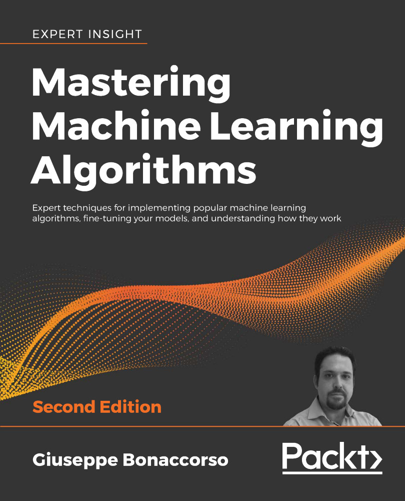
Mastering Machine Learning Algorithms

Mastering Machine Learning Algorithms: Expert techniques for implementing popular machine learning algorithms, fine-tuning your models, and understanding how they work , Second Edition

eBook
₹999.99 ₹3038.99
Paperback
₹3798.99
Paperback + Subscription
₹1000 Monthly

What do you get with a Packt Premium Subscription?

Subscribe today for full access to all titles. After checkout, you’ll receive an eBook credit that you can manually redeem on any title — including this one.
Product feature icon Access to the largest independent learning library in tech. Access this title and thousands more!
Product feature icon Weekly additions on emerging tech and exclusive early access to books as they are being written.
Product feature icon Innovative learning tools, including AI book assistants, code context explainers, and text-to-speech.
Product feature icon A monthly credit and 50% off any future digital purchases.
Table of content icon View table of contents Preview book icon Preview Book

Mastering Machine Learning Algorithms

Loss Functions and Regularization

Loss functions are proxies that allow us to measure the error made by a machine learning model. They define the very structure of the problem to solve, and prepare the algorithm for an optimization step aimed at maximizing or minimizing the loss function. Through this process, we make sure that all our parameters are chosen in order to reduce the error as much as possible. In this chapter, we're going to discuss the fundamental loss functions and their properties. I've also included a dedicated section about the concept of regularization; regularized models are more resilient to overfitting, and can achieve results beyond the limits of a simple loss function.

In particular, we'll discuss:

  • Defining loss and cost functions
  • Examples of cost functions, including mean squared error and the Huber and hinge cost functions
  • Regularization
  • Examples of regularization, including Ridge, Lasso, ElasticNet, and early stopping techniques

We'll begin with some definitions related to loss and cost functions.

Defining loss and cost functions

Many machine learning problems can be expressed throughout a proxy function that measures the training error. The obvious implicit assumption is that, by reducing both training and validation errors, the accuracy increases, and the algorithm reaches its objective.

If we consider a supervised scenario (many considerations hold also for semi-supervised ones), with finite datasets X and Y:

We can define the generic loss function for a single data point as:

J is a function of the whole parameter set and must be proportional to the error between the true label and the predicted label.

A very important property of a loss function is convexity. In many real cases, this is an almost impossible condition; however, it's always useful to look for convex loss functions, because they can be easily optimized through the gradient descent method. We're going to discuss this topic in Chapter 10, Introduction to Time-Series Analysis.

However, for now, it's useful to consider a loss function as an intermediary between our training process and a pure mathematical optimization. The missing link is the complete data. As already discussed, X is drawn from pdata, so it should represent the true distribution. Therefore, when we minimize the loss function, we're considering a potential subset of points, and never the whole real dataset.

In many cases, this isn't a limitation. If the bias is null and the variance is small enough, the resulting model will show a good generalization ability, with high training and validation accuracy; however, considering the data generating process, it's useful to introduce another measure called expected risk:

This value can be interpreted as an average of the loss function over all possible samples drawn from pdata. However, as pdata is generally continuous, it's necessary to consider an expected value and integrate over all possible couples, which is often an intractable problem. The minimization of the expected risk implies the maximization of global accuracy, which, in turn, corresponds to the optimal outcome.

On the other hand, in real-world scenarios we work with a finite number of training samples. Since that's the case, it's preferable to define a cost function, which is often called a loss function as well, and is not to be confused with the log-likelihood:

This is the actual function that we're going to minimize. Divided by the number of samples (a factor that doesn't have any impact) it's also called empirical risk. It's called that because it's an approximation, based on a finite sample X, of the expected risk. In other words, we want to find a set of parameters so that:

When the cost function has more than two parameters, it's very difficult and perhaps even impossible to understand its internal structure. However, we can analyze some potential conditions using a bidimensional diagram:

https://packt-type-cloud.s3.amazonaws.com/uploads/sites/3717/2019/04/1ebd11ad-a339-445d-b020-4358a2c62283.png

Different kinds of points in a bidimensional scenario

The different situations we can observe are:

  • The starting point, where the cost function is usually very high due to the error.
  • Local minima, where the gradient is null and the second derivative is positive. They're candidates for the optimal parameter set, but unfortunately, if the concavity isn't too deep, an inertial movement or noise can easily move the point away.
  • Ridges (or local maxima), where the gradient is null, and the second derivative is negative. They are unstable points, because even minimal perturbation allows escape toward lower-cost areas.
  • Plateaus, or regions where the surface is almost flat and the gradient is close to zero. The only way to escape a plateau is to keep some residual kinetic energy—we're going to discuss this concept when talking about neural optimization algorithms in Chapter 18, Optimizing Neural Networks.
  • Global minimum, the point we want to reach to optimize the cost function.

Even if local minima are likely when the model has a small number of parameters, they become very unlikely when the model has a large number of parameters. In fact, an n-dimensional point is a local minimum for a convex function (and here, we're assuming L to be convex) only if:

The second condition imposes a positive definite Hessian matrix—equivalently, all principal minors made with the first n rows and n columns must be positive—therefore all its eigenvalues must be positive. This probability decreases with the number of parameters ( is an n × n square matrix and has n eigenvalues), and becomes close to zero in deep learning models where the number of weights can be in the order of millions, or even more. The reader interested in a complete mathematical proof can read Dube S., High Dimensional Spaces, Deep Learning and Adversarial Examples, arXiv:1801.00634 [cs.CV].

As a consequence, a more common condition to consider is instead the presence of saddle points, where the eigenvalues have different signs and the orthogonal directional derivatives are null, even if the points are neither local maxima nor local minima. Consider, for example, the following plot:

https://packt-type-cloud.s3.amazonaws.com/uploads/sites/3717/2019/04/232bb91b-4e2c-4610-b76c-c3a55ad2d6eb.png

Saddle point in a three-dimensional scenario

The surface is very similar in shape to a horse saddle, and if we project the point on an orthogonal plane, XZ is a minimum, while on another plane (YZ) it is a maximum. It's straightforward that saddle points are quite dangerous, because many simpler optimization algorithms can slow down and even stop, losing the ability to find the right direction. In Chapter 18, Optimizing Neural Networks, we're going to discuss some methods that are able to mitigate this kind of problem, allowing deep models to converge.

Examples of cost functions

In this section, we'll discuss some common cost functions that are employed in both classification and regression tasks. Some of them will be repeatedly adopted in our examples over the next few chapters, particularly when we're discussing training processes in shallow and deep neural networks.

Mean squared error

Mean squared error is one of the most common regression cost functions. Its generic expression is:

This function is differentiable at every point of its domain and it's convex, so it can be optimized using the stochastic gradient descent (SGD) algorithm. This cost function is fundamental in regression analysis using the Ordinary or Generalized Least Square algorithms, where, for example, it's possible to prove that the estimators are always unbiased.

However, there's a drawback when employing it in regression tasks with outliers. Its value is always quadratic, and therefore, when the distance between the prediction and an actual outlier value is large, the relative error is large, and this can lead to an unacceptable correction.

Huber cost function

As explained, mean squared error isn't robust to outliers, because it's always quadratic, independent of the distance between actual value and prediction. To overcome this problem, it's possible to employ the Huber cost function, which is based on threshold tH, so that for distances less than tH its behavior is quadratic, while for a distance greater than tH it becomes linear, reducing the entity of the error and thereby reducing the relative importance of the outliers.

The analytical expression is:

Hinge cost function

This cost function is adopted by Support Vector Machine (SVM) algorithms, where the goal is to maximize the distance between the separation boundaries, where the support vectors lie. Its analytic expression is:

Contrary to the other examples, this cost function is not optimized using classic SGD methods, because it's not differentiable when:

For this reason, SVM algorithms are optimized using quadratic programming techniques.

Categorical cross-entropy

Categorical cross-entropy is the most diffused classification cost function, adopted by logistic regression and the majority of neural architectures. The generic analytical expression is:

This cost function is convex and can easily be optimized using SGD techniques. According to information theory, the entropy of a distribution p is a measure of the amount of uncertainty—expressed in bit if is used and in nat is natural logarithm is employed—carried by a particular probability distribution. For example, if we toss a fair coin, then according to a Bernoulli distribution. Therefore, the entropy of such a discrete distribution is:

The uncertainty is equal to 1 bit, which means that before any experiment there are 2 possible outcomes, which is obvious. What happens if we know that the coin is loaded, and P(Head) = 0.1 and P(Tail) = 0.9? The entropy is now:

As our uncertainty is now very low—we know that in 90% of the cases, the outcome will be tails—the entropy is less than half a bit. The concept must be interpreted as a continuous measure, which means that a single outcome is very likely to appear. The extreme case when P(Head) → 0 and P(Tail) → 1 asymptotically requires 0 bits, because there's no more uncertainty and the probability distribution is degenerate.

The concept of entropy, as well as cross-entropy and other information theory formulas, can be extended to continuous distributions using an integral instead of a sum. For example, the entropy of a normal distribution is . In general, the entropy is proportional to the variance or to the spread of the distribution.

This is an intuitive concept, in fact; the larger the variance, the larger the region in which the potential outcomes have a similar probability to be selected. As the uncertainty grows when the potential set of candidate outcomes does, the price in bits or nats we need to pay to remove the uncertainty increases. In the example of the coin, we needed to pay 1 bit for a fair outcome and only 0.47 bit when we already knew that P(Tail) = 0.9; our uncertainty was quite a lot lower.

Analogously, cross-entropy is defined between two distributions p and q:

Let's suppose that p is the data generating process we are working with. What's the meaning of H(P, q)? Considering the expression, what we're doing is computing the expected value , while the entropy computed the expected value . Therefore, if q is an approximation of p, the cross-entropy measures the additional uncertainty that we are introducing when using the model q instead of the original data generating process. It's not difficult to understand that we increase the uncertainty by only using an approximation of the true underlying process.

In fact, if we're training a classifier, our goal is to create a model whose distribution is as similar as possible to pdata. This condition can be achieved by minimizing the Kullback-Leibler divergence between the two distributions:

In the previous expression, pM is the distribution generated by the model. Now, if we rewrite the divergence, we get:

The first term is the entropy of the data generating distribution, and it doesn't depend on the model parameters, while the second one is the cross-entropy. Therefore, if we minimize the cross-entropy, we also minimize the Kullback-Leibler divergence, forcing the model to reproduce a distribution that is very similar to pdata. That means that we are reducing the additional uncertainty that was induced by the approximation. This is a very elegant explanation as to why the cross-entropy cost function is an excellent choice for classification problems.

Regularization

When a model is ill-conditioned or prone to overfitting, regularization offers some valid tools to mitigate the problems. From a mathematical viewpoint, a regularizer is a penalty added to the cost function, to impose an extra condition on the evolution of the parameters:

The parameter controls the strength of the regularization, which is expressed through the function . A fundamental condition on is that it must be differentiable so that the new composite cost function can still be optimized using SGD algorithms. In general, any regular function can be employed; however, we normally need a function that can contrast the indefinite growth of the parameters.

To understand the principle, let's consider the following diagram:

https://packt-type-cloud.s3.amazonaws.com/uploads/sites/3717/2019/05/IMG_49.png

Interpolation with a linear curve (left) and a parabolic one (right)

In the first diagram, the model is linear and has two parameters, while in the second one, it is quadratic and has three parameters. We already know that the second option is more prone to overfitting, but if we apply a regularization term, it's possible to avoid the growth of the first quadratic parameter and transform the model into a linearized version.

Of course, there's a difference between choosing a lower-capacity model and applying a regularization constraint. In the first case, we are renouncing the possibility offered by the extra capacity with a consequent risk of large bias, while with regularization we keep the same model but optimize it to reduce the variance and only slightly increase the bias. I hope it's clear that regularization always leads to a suboptimal model M' and, in particular, if the original M is unbiased, M' will be biased proportionally to and to the kind of regularization used.

Generally speaking, if the absolute minimum of a cost function with respect to a training set is copt, any model with c > copt is suboptimal. This means that the training error is larger, but the generalization error might be better controlled.

In fact, a perfectly trained model could have learned the structure of the training set and reached a minimum loss, but, when a new sample is checked, the performance is much worse.

Even if it's not very mathematically rigorous, we can say that regularization often acts as a brake that avoids perfect convergence. By doing this, it keeps the model in a region where the generalization error is lower, which is, generally, the main objective of machine learning. Hence, this extra penalty can be accepted in the context of the bias-variance trade-off.

A small bias can be acceptable when it's the consequence of a drastic variance reduction (that is, a smaller generalization error); however, I strongly suggest that you don't employ regularization as a black-box technique, but instead to check (for example, using cross-validation) which value yields the optimal result, intended as a trade-off.

Examples of Regularization Techniques

At this point, we can explore the most common regularization techniques and discuss their properties.

L2 or Ridge regularization

L2 or Ridge regularization, also known as Tikhonov regularization, is based on the squared L2-norm of the parameter vector:

This penalty avoids infinite growth of the parameters—for this reason, it's also known as weight shrinkage—and it's particularly useful when the model is ill-conditioned, or there is multicollinearity due to the fact that the samples are not completely independent, which is a relatively common condition.

In the following diagram, we see a schematic representation of the Ridge regularization in a bidimensional scenario:

https://packt-type-cloud.s3.amazonaws.com/uploads/sites/3717/2019/04/af342c73-233f-42a7-b7c0-f724fe9c9865.png 

Ridge (L2) regularization

The zero-centered circle represents the Ridge boundary, while the shaded surface is the original cost function. Without regularization, the minimum (w1, w2) has a magnitude (for example, the distance from the origin) which is about double the one obtained by applying a Ridge constraint, confirming the expected shrinkage.

When applied to regressions solved with the Ordinary Least Squares (OLS) algorithm, it's possible to prove that there always exists a Ridge coefficient, so that the weights are shrunk with respect to the OLS ones. The same result, with some restrictions, can be extended to other cost functions.

Moreover, Andrew Ng (in Ng A. Y., Feature selection, L1 vs. L2 regularization, and rotational invariance, ICML, 2004) proved that L2 regularization, applied to the majority of classification algorithms, allows us to obtain rotational invariance. In other words, if the training set is rotated, a regularized model will yield the same prediction distribution as the original one. Another fundamental aspect to remember is that L2-regularization shrinks the weights independent of the scale of the data. Therefore, if the features have different scales, the result may be worse than expected.

It's easy to understand this concept by considering a simple linear model with two variables, y = ax1 + bx1 + c. As the L2 has a single control coefficient, the effect will be the same on both a and b (excluding the intercept c). If and , the shrinkage will affect x1 much more than x2.

For this reason, we recommend scaling the dataset before applying the regularization. Other important properties of this method will be discussed throughout the book, when specific algorithms are introduced.

L1 or Lasso regularization

L1 or Lasso regularization is based on the L1-norm of the parameter vector:

While Ridge shrinks all the weights inversely proportionally to their importance, Lasso can shift the smallest weight to zero, creating a sparse parameter vector.

The mathematical proof is beyond the scope of this book; however, it's possible to understand it intuitively by considering the following bidimensional diagram:

https://packt-type-cloud.s3.amazonaws.com/uploads/sites/3717/2019/04/4902bfec-7cac-4364-8467-ee03581729ea.png

Lasso (L1) regularization

The zero-centered square represents the Lasso boundaries in a bidimensional scenario (it will be a hyperdiamond in ). If we consider a generic line, the probability of that line being tangential to the square is higher at the corners, where at least one parameter is null—exactly one parameter in a bidimensional scenario. In general, if we have a vectorial convex function f(x) (we provide a definition of convexity in Chapter 7, Advanced Clustering and Unsupervised Models), we can define:

As any Lp-norm is convex, as well as the sum of convex functions, is also convex. The regularization term is always non-negative, and therefore the minimum corresponds to the norm of the null vector.

When minimizing , we also need to consider the contribution of the gradient of the norm in the ball centered in the origin, where the partial derivatives don't exist. Increasing the value of p, the norm becomes smoothed around the origin, and the partial derivatives approach zero for .

On the other hand, excluding the L0-norm and all the norms with allows an even stronger sparsity, but is non-convex (even if L0 is currently employed in the quantum algorithm QBoost). With p = 1 the partial derivatives are always +1 or -1, according to the sign of . Therefore, it's easier for the L1-norm to push the smallest components to zero, because the contribution to the minimization (for example, with gradient descent) is independent of xi, while an L2-norm decreases its speed when approaching the origin.

This is a non-rigorous explanation of the sparsity achieved using the L1-norm. In practice, we also need to consider the term , which bounds the value of the global minimum; however, it may help the reader to develop an intuitive understanding of the concept. It's possible to find further, more mathematically rigorous details in Sra S., Nowozin S., Wright S. J. (edited by), Optimization for Machine Learning, The MIT Press, 2011.

Lasso regularization is particularly useful when a sparse representation of a dataset is needed. For example, we could be interested in finding the feature vectors corresponding to a group of images. As we expect to have many features, but only a subset of those features present in each image, applying the Lasso regularization allows us to force all the smallest coefficients to become null, which helps us by suppressing the presence of the secondary features.

Another potential application is latent semantic analysis, where our goal is to describe the documents belonging to a corpus in terms of a limited number of topics. All these methods can be summarized in a technique called sparse coding, where the objective is to reduce the dimensionality of a dataset by extracting the most representative atoms, using different approaches to achieve sparsity.

Another important property of L1 regularization concerns its ability to perform an implicit feature selection, induced by the sparsity. In a generic scenario, a dataset can also include irrelevant features that don't contribute to increasing the accuracy of the classification. This can happen because real-world datasets are often redundant, and the data collectors are more interested in their readability than in their usage for analytical purposes. There are many techniques (some of them are described in Bonaccorso G., Machine Learning Algorithms, Second Edition, Packt, 2018) that can be employed to select only those features that really transport unique pieces of information and discard the remaining ones; however, L1 is particularly helpful.

First of all, it's automatic and no preprocessing steps are required. This is extremely useful in deep learning. Moreover, as Ng pointed out in the aforementioned paper, if a dataset contains n features, the minimum number of samples required to increase the accuracy over a predefined threshold is affected by the logarithm of the number of redundant or irrelevant features.

This means, for example, that if dataset X contains 1000 points and the optimal accuracy is achieved with this sample size when all the features are informative when k < p features are irrelevant, we need approximately 1000 + O(log k) samples. This is a simplification of the original result; for example, if p = 5000 and 500 features are irrelevant, assuming the simplest case, we need about data points.

Such a result is very important because it's often difficult and expensive to obtain a large number of new samples, in particular when they are obtained in experimental contexts (for example, social sciences, pharmacological research, and so on). Before moving on, let's consider a synthetic dataset containing 500 points with only five informative features:

from sklearn.datasets import make_classification
from sklearn.preprocessing import StandardScaler
X, Y = make_classification(n_samples=500, n_classes=2, n_features=10, n_informative=5, 
                           n_redundant=3, n_clusters_per_class=2, random_state=1000)
ss = StandardScaler()
X_s = ss.fit_transform(X)

We can now fit two logistic regression instances with the whole dataset: the first one using the L2 regularization and the second one using L1. In both cases, the strength is kept fixed:

from sklearn.linear_model import LogisticRegression
lr_l2 = LogisticRegression(solver='saga', penalty='l2', C=0.25, random_state=1000)
lr_l1 = LogisticRegression(solver='saga', penalty='l1', C=0.25, random_state=1000)
lr_l2.fit(X_s, Y)
lr_l1.fit(X_s, Y)

It's possible to see that, in both cases, the 10-fold cross-validation yields approximately the same average accuracy. However, in this case, we are more interested in checking the feature selection properties of L1; therefore we are going to compare the 10 coefficients of the two models, available as an instance variable coef_. The results are shown in the following figure:

https://packt-type-cloud.s3.amazonaws.com/uploads/sites/3717/2019/05/IMG_50.png

Logistic regression coefficients with L1 (left) and L2 (right) regularizations

As you can see, L2 regularization tends to shrink all coefficients almost uniformly, excluding the dominance of 9 and 10, while L1 performs a feature selection, by keeping only 5 non-null coefficients. This result is coherent with the structure of the dataset, in that it contains only 5 informative features and, therefore, a good classification algorithm can get rid of the remaining ones.

It's helpful to remember that we often need to create explainable models. That is to say, we often need to create models whose output can be immediately traced back to its causes. When there are many parameters, this task becomes more difficult. The usage of Lasso allows us to exclude all those features whose importance is secondary with respect to a primary group. In this way, the resulting model is smaller, and definitely more explainable.

As a general suggestion, in particular when working with linear models, I invite the reader to perform a feature selection to remove all non-determinant factors; and L1 regularization is an excellent choice that avoids an additional preprocessing step.

Having discussed the main properties of both L1 and L2 regularizations, we can now explain how to combine them in order to exploit the respective benefits.

ElasticNet

In many real cases, it's useful to apply both Ridge and Lasso regularization in order to force weight shrinkage and a global sparsity. It is possible by employing the ElasticNet regularization, defined as:

The strength of each regularization is controlled by the parameters and . ElasticNet can yield excellent results whenever it's necessary to mitigate overfitting effects, while encouraging sparsity. We're going to apply all these regularization techniques when we discuss deep learning architectures.

Early stopping

Even though it's a pure regularization technique, early stopping is often considered a last resort when all other approaches to prevent overfitting, and maximize validation accuracy, fail. In many cases, above all in deep learning scenarios even though it can also happen with SVMs and other simpler classifiers, it's possible to observe a typical behavior of the training process, considering both training and the validation cost functions:

https://packt-type-cloud.s3.amazonaws.com/uploads/sites/3717/2019/04/7b96eec9-cac9-4134-b959-2c8ed73f2584.png

Example of early stopping before the beginning of the ascending phase of a U-curve

During the first epochs, both costs decrease, but it can happen that after a threshold epoch es, the validation cost starts increasing. If we continue with the training process, this results in overfitting the training set and increasing the variance.

For this reason, when there are no other options, it's possible to prematurely stop the training process. In order to do so, it's necessary to store the last parameter vector before the beginning of a new iteration and, in the case of no improvements or the accuracy worsening, to stop the process and recover the last set of parameters.

As explained, this procedure must never be considered as the best choice, because a better model or an improved dataset could yield higher performances. With early stopping, there's no way to verify alternatives, therefore it must be adopted only at the last stage of the process and never at the beginning.

Many deep learning frameworks such as Keras include helpers to implement early stopping callbacks. However, it's important to check whether the last parameter vector is the one stored before the last epoch or the one corresponding to es. In this case, it could be helpful to repeat the training process, stopping it at the epoch previous to es, where the minimum validation cost has been achieved.

Summary

In this chapter, we introduced the loss and cost functions, first as proxies of the expected risk, and then we detailed some common situations that can be experienced during an optimization problem. We also exposed some common cost functions, together with their main features and specific applications.

In the last part, we discussed regularization, explaining how it can mitigate the effects of overfitting and induce sparsity. In particular, the employment of Lasso can help the data scientist to perform automatic feature selection by forcing all secondary coefficients to become equal to 0.

In the next chapter, Chapter 3, Introduction to Semi-Supervised Learning, we're going to introduce semi-supervised learning, focusing our attention on the concepts of transductive and inductive learning.

Further reading

  • Darwiche A., Human-Level Intelligence or Animal-Like Abilities?, Communications of the ACM, Vol. 61, 10/2018
  • Crammer K., Kearns M., Wortman J., Learning from Multiple Sources, Journal of Machine Learning Research, 9/2008
  • Mohri M., Rostamizadeh A., Talwalkar A., Foundations of Machine Learning, Second edition, The MIT Press, 2018
  • Valiant L., A theory of the learnable, Communications of the ACM, 27, 1984
  • Ng A. Y., Feature selection, L1 vs. L2 regularization, and rotational invariance, ICML, 2004
  • Dube S., High Dimensional Spaces, Deep Learning and Adversarial Examples, arXiv:1801.00634 [cs.CV]
  • Sra S., Nowozin S., Wright S. J. (edited by), Optimization for Machine Learning, The MIT Press, 2011
  • Bonaccorso G., Machine Learning Algorithms, Second Edition, Packt, 2018
Left arrow icon Right arrow icon
Download code icon Download Code

Key benefits

  • Updated to include new algorithms and techniques
  • Code updated to Python 3.8 & TensorFlow 2.x
  • New coverage of regression analysis, time series analysis, deep learning models, and cutting-edge applications

Description

Mastering Machine Learning Algorithms, Second Edition helps you harness the real power of machine learning algorithms in order to implement smarter ways of meeting today's overwhelming data needs. This newly updated and revised guide will help you master algorithms used widely in semi-supervised learning, reinforcement learning, supervised learning, and unsupervised learning domains. You will use all the modern libraries from the Python ecosystem – including NumPy and Keras – to extract features from varied complexities of data. Ranging from Bayesian models to the Markov chain Monte Carlo algorithm to Hidden Markov models, this machine learning book teaches you how to extract features from your dataset, perform complex dimensionality reduction, and train supervised and semi-supervised models by making use of Python-based libraries such as scikit-learn. You will also discover practical applications for complex techniques such as maximum likelihood estimation, Hebbian learning, and ensemble learning, and how to use TensorFlow 2.x to train effective deep neural networks. By the end of this book, you will be ready to implement and solve end-to-end machine learning problems and use case scenarios.

Who is this book for?

This book is for data science professionals who want to delve into complex ML algorithms to understand how various machine learning models can be built. Knowledge of Python programming is required.

What you will learn

  • Understand the characteristics of a machine learning algorithm
  • Implement algorithms from supervised, semi-supervised, unsupervised, and RL domains
  • Learn how regression works in time-series analysis and risk prediction
  • Create, model, and train complex probabilistic models
  • Cluster high-dimensional data and evaluate model accuracy
  • Discover how artificial neural networks work – train, optimize, and validate them
  • Work with autoencoders, Hebbian networks, and GANs

Product Details

Country selected
Publication date, Length, Edition, Language, ISBN-13
Publication date : Jan 31, 2020
Length: 798 pages
Edition : 2nd
Language : English
ISBN-13 : 9781838820299
Vendor :
Google
Category :
Languages :
Tools :

What do you get with a Packt Premium Subscription?

Subscribe today for full access to all titles. After checkout, you’ll receive an eBook credit that you can manually redeem on any title — including this one.
Product feature icon Access to the largest independent learning library in tech. Access this title and thousands more!
Product feature icon Weekly additions on emerging tech and exclusive early access to books as they are being written.
Product feature icon Innovative learning tools, including AI book assistants, code context explainers, and text-to-speech.
Product feature icon A monthly credit and 50% off any future digital purchases.

Product Details

Publication date : Jan 31, 2020
Length: 798 pages
Edition : 2nd
Language : English
ISBN-13 : 9781838820299
Vendor :
Google
Category :
Languages :
Tools :

Packt Subscriptions

See our plans and pricing
Modal Close icon
₹800 billed monthly
Feature tick icon Unlimited access to Packt's library of 7,000+ practical books and videos
Feature tick icon Constantly refreshed with 50+ new titles a month
Feature tick icon Exclusive Early access to books as they're written
Feature tick icon Solve problems while you work with advanced search and reference features
Feature tick icon Offline reading on the mobile app
Feature tick icon Simple pricing, no contract
₹4500 billed annually
Feature tick icon Unlimited access to Packt's library of 7,000+ practical books and videos
Feature tick icon Constantly refreshed with 50+ new titles a month
Feature tick icon Exclusive Early access to books as they're written
Feature tick icon Solve problems while you work with advanced search and reference features
Feature tick icon Offline reading on the mobile app
Feature tick icon Choose a DRM-free eBook or Video every month to keep
Feature tick icon PLUS own as many other DRM-free eBooks or Videos as you like for just ₹400 each
Feature tick icon Exclusive print discounts
₹5000 billed in 18 months
Feature tick icon Unlimited access to Packt's library of 7,000+ practical books and videos
Feature tick icon Constantly refreshed with 50+ new titles a month
Feature tick icon Exclusive Early access to books as they're written
Feature tick icon Solve problems while you work with advanced search and reference features
Feature tick icon Offline reading on the mobile app
Feature tick icon Choose a DRM-free eBook or Video every month to keep
Feature tick icon PLUS own as many other DRM-free eBooks or Videos as you like for just ₹400 each
Feature tick icon Exclusive print discounts

Frequently bought together


Stars icon
Total 12,215.97
Mastering Machine Learning Algorithms
₹3798.99
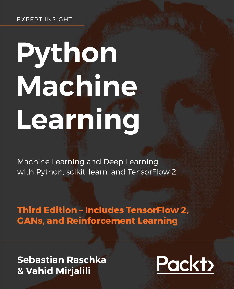
Python Machine Learning
₹4096.99
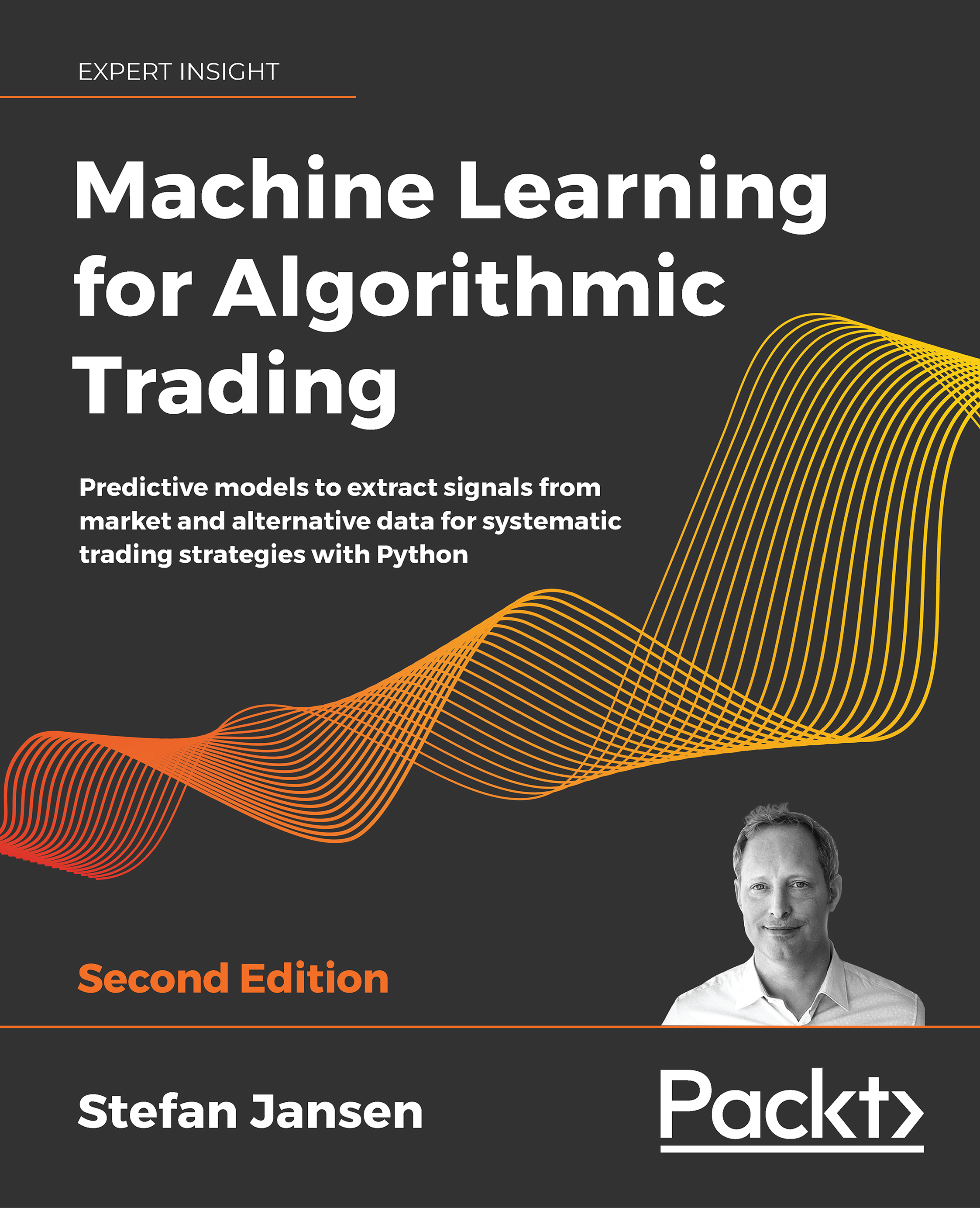
Machine Learning for Algorithmic Trading
₹4319.99
Total 12,215.97 Stars icon

Table of Contents

27 Chapters
Machine Learning Model Fundamentals Chevron down icon Chevron up icon
Loss Functions and Regularization Chevron down icon Chevron up icon
Introduction to Semi-Supervised Learning Chevron down icon Chevron up icon
Advanced Semi-Supervised Classification Chevron down icon Chevron up icon
Graph-Based Semi-Supervised Learning Chevron down icon Chevron up icon
Clustering and Unsupervised Models Chevron down icon Chevron up icon
Advanced Clustering and Unsupervised Models Chevron down icon Chevron up icon
Clustering and Unsupervised Models for Marketing Chevron down icon Chevron up icon
Generalized Linear Models and Regression Chevron down icon Chevron up icon
Introduction to Time-Series Analysis Chevron down icon Chevron up icon
Bayesian Networks and Hidden Markov Models Chevron down icon Chevron up icon
The EM Algorithm Chevron down icon Chevron up icon
Component Analysis and Dimensionality Reduction Chevron down icon Chevron up icon
Hebbian Learning Chevron down icon Chevron up icon
Fundamentals of Ensemble Learning Chevron down icon Chevron up icon
Advanced Boosting Algorithms Chevron down icon Chevron up icon
Modeling Neural Networks Chevron down icon Chevron up icon
Optimizing Neural Networks Chevron down icon Chevron up icon
Deep Convolutional Networks Chevron down icon Chevron up icon
Recurrent Neural Networks Chevron down icon Chevron up icon
Autoencoders Chevron down icon Chevron up icon
Introduction to Generative Adversarial Networks Chevron down icon Chevron up icon
Deep Belief Networks Chevron down icon Chevron up icon
Introduction to Reinforcement Learning Chevron down icon Chevron up icon
Advanced Policy Estimation Algorithms Chevron down icon Chevron up icon
Other Books You May Enjoy Chevron down icon Chevron up icon
Index Chevron down icon Chevron up icon

Customer reviews

Top Reviews
Rating distribution
Full star icon Full star icon Full star icon Full star icon Empty star icon 4
(12 Ratings)
5 star 50%
4 star 25%
3 star 8.3%
2 star 8.3%
1 star 8.3%
Filter icon Filter
Top Reviews

Filter reviews by


hawkinflight Aug 13, 2020
Full star icon Full star icon Full star icon Full star icon Full star icon 5
The book covers a lot of methods, as can be seen in the table of contents. This provides a nice breadth. What is really nice, is that before getting into any of the methods, the author starts with a chapter on ML Model Fundamentals. In this chapter, he presents not just the how's but also the why's of scaling data before modeling. He also talks about model capacity, bias and variance of an estimator, and how these relate to under or over fitting a model. Recently, I have heard two things during presentations: 1) "I won't go over scaling, because I think we all know when to apply these transformations" 2) "I don't even know what you're talking about" when asked about a bias/variance trade-off. I think it's great to have the opportunity to read a practitioner's explanation of these matters. He also talks about the options for splitting a data set into portions: 1) training, validation, and test portions, or 2) just into training and test portions, or 3) using a cross-validation approach. I have taken an ML class on Coursera where the first option was used, and the others weren't mentioned. It's nice to see all three here. He helps the reader by noting that some topics he's introducing will be discussed in more detail in the next few chapters. That's nice because questions start arising in your head, and then you read that and know there's more detail and answers coming, so just relax, and look forward.There are nice plots and Python code snippets throughout. It's helpful that each chapter ends with a summary and list of references.A lot of times we hear "supervised" or "unsupervised". It's nice that the book has three chapters on "semi-supervised" learning. In the Graph-Based Semi-Supervised Learning chapter, there is a "t-distributed stochastic neighbor embedding" (t-SNE) example, which is a topic I was curious about.
Amazon Verified review Amazon
Alfred H. Mar 06, 2020
Full star icon Full star icon Full star icon Full star icon Full star icon 5
I look at algorithms like appliances in a department store. Each has a particular use-case and purpose. For instance, depending on your individual needs while shopping for appliances most often stop to glance at the specs then at the cost to see if a particular unit suits their needs.Few ever think to build the appliance from scratch but rather by one already made to serve their needs progressively adopting it as an augmentation to everyday life. Even easier is when these items can be cataloged in one place, shopped, and put into use immediately (think Sears catalog of 1888). In its first catalog, Sears sold jewelry and watches. The directories grew in popularity, and with time different products were added and tested, even whole houses!While algorithms are not a new thing, thanks to the father of algebra: Abdullah Muhammad bin Musa al-Khwarizmi, it should NOT be challenging to catalog them. This book one of the best, like it, does that facilitating faster solutioning to get to the point of solving problems using built appliances (machine intelligence: algorithms).
Amazon Verified review Amazon
Thom Ives, Ph.D. May 26, 2020
Full star icon Full star icon Full star icon Full star icon Full star icon 5
Our exciting field of data science (DS) is exploding, and it’s hard to keep up with all of it. We each become extremely focused on our specific work in our current roles, and we are each funneled into specialized areas to solve specific challenges. After a long battle to deliver your great DS tool to production, your next challenge arrives. It seems this problem will require a DS method that you haven’t used since college. Maybe you’re not even sure, which DS method will best address your problem. Regardless, once you decide on a method of modeling, you have limited time to master it. You still need to collect, refine, and condition your data for that method. You must also master how to fight through the training of your chosen model. You’d seek help from your fellow DS’s, but they’re in the situation you just left.Now enters Giuseppe Bonaccorso - a DS friend with a corpus of DS methods that provide adequate mathematical overviews, explanations, and python code applied to substantial examples to get you up to speed quickly. I believe in keeping multiple sources at hand for learning / reviewing any methods. In that spirit, I'm relieved to have Giuseppe's book in my library. In a mere 750+ pages, he takes you on a tour of important methods that, while they won't make you an expert in the foundational mathematics for each method, they won't leave you blind in those respects either. I especially appreciate the references to foundational papers for each method following every group of methods for when we might need or want to go deeper. If you estimate that your library could be enhanced by such a substantial book as I've described, I believe you'd be well benefited by Giuseppe's book. He even manages to provide a good review of reinforced learning that, in my opinion, is extremely challenging to teach clearly.An important note is that this book does not cover natural language processing. In my experience, NLP would require another 750+ pages if it were to be covered as well as the methods that Giuseppe has covered. However, this is the only major field that he skips, and he does relate areas of that field to the techniques that he covers.
Amazon Verified review Amazon
TD59 Jun 13, 2021
Full star icon Full star icon Full star icon Full star icon Full star icon 5
I have used this book (1st and 2nd edition) in my Machine Learning class for a couple of years. Together with the Raschka and Mirjalili book (Python Machine Learning), Bonnacorso's provides a solid foundation for understanding the key algorithms, how they work, and how to fine-tune them. Both amanuals re required in my class and my students have only had positive feedback about both books. They are complementary as Bonnacorso does not cover some topics such as Natural Language Processing compared with Raschka, for instance.
Amazon Verified review Amazon
Duubar Villalobos Feb 19, 2020
Full star icon Full star icon Full star icon Full star icon Full star icon 5
As Giuseppe Bonaccorso expresses in this book, "It's always possible to join scientific rigor with an artistic approach." This book offers a great resource to dust off those concepts for the advance practitioners or to learn the fundamentals for those willing to master their ML algorithms artistically.I've been reading this book for over a week by now, and I like how Giuseppe explains important theoretical concepts related to machine learning models, bias, variance, overfitting, underfitting, data normalization, scaling, and so on.Even though this book requires a solid knowledge of essential machine learning topics and familiarity with Python programming language, don't be discouraged. I found out that this book provides the best first-hand experiential advice that someone can provide for someone willing to learn. Moreover, given the complexity of some subjects, proper mathematical training is desirable, but the willingness to learn outweighs it.If you are looking to get great advice and insights from an expert, this book is for you. My recommendation is not to rush over the concepts. As I am reading --still not finished since it's 800 pages, it makes me reflect on my problem-solving styles and helps me identify areas of opportunity for improvement.I have to thank Giuseppe for taking his time to think, sort his thoughts, write, and for sharing his knowledge and experiences for us to become better practitioners.
Amazon Verified review Amazon
Get free access to Packt library with over 7500+ books and video courses for 7 days!
Start Free Trial

FAQs

What is included in a Packt Premium subscription? Chevron down icon Chevron up icon

A subscription provides you with full access to view all Packt and licnesed content online, this includes exclusive access to Early Access titles. Depending on the tier chosen you can also earn credits and discounts to use for owning content

What are credits? Chevron down icon Chevron up icon

Credits can be used to buy books DRM free, the same way that you would pay for a book. Your credits can be found in the subscription homepage - subscription.packtpub.com - clicking on ‘the my’ library dropdown and selecting ‘credits’. You'll get one to use immediately after checkout, and then every time you renew. You require an active subscription to use your credits, once used you keep the title forever.

How can I cancel my subscription? Chevron down icon Chevron up icon

To cancel your subscription with us simply go to the account page - found in the top right of the page or at https://subscription.packtpub.com/my-account/subscription - From here you will see the ‘cancel subscription’ button in the grey box with your subscription information in. You can cancel at anytime, you will keep access for the remaining period you have paid for. On the date of cancellation you will lose all access to online content, along with any unused credits.

What happens if an Early Access Course is cancelled? Chevron down icon Chevron up icon

Projects are rarely cancelled, but sometimes it's unavoidable. If an Early Access course is cancelled or excessively delayed, you can exchange your purchase for another course. For further details, please contact us here.

Where can I send feedback about an Early Access title? Chevron down icon Chevron up icon

If you have any feedback about the product you're reading, or Early Access in general, then please fill out a contact form here and we'll make sure the feedback gets to the right team. 

Can I download the code files for Early Access titles? Chevron down icon Chevron up icon

We try to ensure that all books in Early Access have code available to use, download, and fork on GitHub. This helps us be more agile in the development of the book, and helps keep the often changing code base of new versions and new technologies as up to date as possible. Unfortunately, however, there will be rare cases when it is not possible for us to have downloadable code samples available until publication.

When we publish the book, the code files will also be available to download from the Packt website.

How accurate is the publication date? Chevron down icon Chevron up icon

The publication date is as accurate as we can be at any point in the project. Unfortunately, delays can happen. Often those delays are out of our control, such as changes to the technology code base or delays in the tech release. We do our best to give you an accurate estimate of the publication date at any given time, and as more chapters are delivered, the more accurate the delivery date will become.

How will I know when new chapters are ready? Chevron down icon Chevron up icon

We'll let you know every time there has been an update to a course that you've bought in Early Access. You'll get an email to let you know there has been a new chapter, or a change to a previous chapter. The new chapters are automatically added to your account, so you can also check back there any time you're ready and download or read them online.

I am a Packt subscriber, do I get Early Access? Chevron down icon Chevron up icon

Yes, all Early Access content is fully available through your subscription. You will need to have a paid for or active trial subscription in order to access all titles.

How is Early Access delivered? Chevron down icon Chevron up icon

Early Access is currently only available as a PDF or through our online reader. As we make changes or add new chapters, the files in your Packt account will be updated so you can download them again or view them online immediately.

How do I buy Early Access content? Chevron down icon Chevron up icon

Early Access is a way of us getting our content to you quicker, but the method of buying the Early Access course is still the same. Just find the course you want to buy, go through the check-out steps, and you’ll get a confirmation email from us with information and a link to the relevant Early Access courses.

What is Early Access? Chevron down icon Chevron up icon

Keeping up to date with the latest technology is difficult; new versions, new frameworks, new techniques. This feature gives you a head-start to our content, as it's being created. With Early Access you'll receive each chapter as it's written, and get regular updates throughout the product's development, as well as the final course as soon as it's ready.We created Early Access as a means of giving you the information you need, as soon as it's available. As we go through the process of developing a course, 99% of it can be ready but we can't publish until that last 1% falls in to place. Early Access helps to unlock the potential of our content early, to help you start your learning when you need it most. You not only get access to every chapter as it's delivered, edited, and updated, but you'll also get the finalized, DRM-free product to download in any format you want when it's published. As a member of Packt, you'll also be eligible for our exclusive offers, including a free course every day, and discounts on new and popular titles.

Modal Close icon
Modal Close icon