From the typical ML application process depicted in Figure 1.1, you can see that ML has a broad range of applications. However, ML algorithms are only a small part of a bigger ecosystem with a lot of moving parts, and yet ML is transforming lives around the world today:

Deployed ML applications usually start with a process of data collection that uses sensors of different types, such as cameras, lasers, spectroscopes, or other types of direct access to data, including local and remote databases, big or small. In the simplest of cases, input can be gathered through a computer keyboard or smartphone screen taps. At this stage, the data collected or sensed is considered to be raw data.

Raw data is usually preprocessed before presenting it to an ML model. Raw data is rarely the actual input to ML algorithms, unless the ML model is meant to find a rich representation of the raw data, and later be used as input to another ML algorithm. In other words, there are some ML algorithms that are specifically used as preprocessing agents and they are not at all related to a main ML model that will classify or regress on the preprocessed data. In a general sense, this data preprocessing stage aims to convert raw data into arrays or matrices with specific data types. Some popular preprocessing strategies include the following:

• Word-to-vector conversions, for example, using GloVe or Word2Vec
• Sequence-to-vector or sequence-to-matrix strategies
• Value range normalization, for example, (0, 255) to (0.0, 1.0)
• Statistical value normalization, for example, to have zero mean and unit variance

Once these preprocessing measures take place, most ML algorithms can use the data. However, it must be noted that the preprocessing stage is not trivial, it requires advanced knowledge and skills with respect to operating systems and sometimes even electronics. In a general sense, a real ML application has a long pipeline touching different aspects of computer science and engineering.

Mathematically speaking, the processed data as a whole is referred to using the uppercase, bold font, letter X, which has N rows (or data points). If we want to refer to the specific i-th element (or row) of the dataset, we would do that by writing: X_i. The dataset will have d columns and they are usually called features. One way to think about the features is as dimensions. For example, if the dataset has two features, height and weight, then you could represent the entire dataset using a two-dimensional plot. The first dimension, x₁, (height) can be the horizontal axis, while the second dimension, x₂, (weight) can be the vertical axis, as depicted in Figure 1.2:

During production, when the data is presented to an ML algorithm, a series of tensor products and additions will be executed. Such vectorial operations are usually transformed or normalized using non-linear functions. This is then followed by more products and additions, more non-linear transformations, temporary storage of intermediate values, and finally producing the desired output that corresponds to the input. For now, you can think of this process as an ML black box that will be revealed as you continue reading.

The output that the ML produces in correspondence to the input usually requires some type of interpretation, for example, if the output is a vector of probabilities of objects being classified to belong to a group or to another, then that may need to be interpreted. You may need to know how low the probabilities are in order to account for uncertainty, or you may need to know how different are the probabilities to account for even more uncertainty. The output processing serves as the connecting factor between ML and the decision-making world through the use of business rules. These rules can be, for example, if-then rules such as, "If the predicted probability of the maximum is twice as large as the second maximum, then issue a prediction; otherwise, do not proceed to make a decision." Or they can be formula-based rules or more complex systems of equations.

Finally, in the decision-making stage, the ML algorithm is ready to interact with the world by turning on a light bulb through an actuator, or to buy stock if the prediction is not uncertain, by alerting a manager that the company will run out of inventory in three days and they need to buy more items, or by sending an audio message to a smartphone speaker saying, "Here is the route to the movie theater" and opening a maps application through an application programming interface (API) call or operating system (OS) commands.

This is a broad overview of the world of ML systems when they are in production. However, this assumes that the ML algorithm is properly trained and tested, which is the easy part, trust me. At the end of the book, you will be skilled in training highly complex, deep learning algorithms but, for now, let us introduce the generic training process.

A typical preprocessed dataset is formally defined as follows:

Where y is the desired output corresponding to the input vector x. So, the motivation of ML is to use the data to find linear and non-linear transformations over x using highly complex tensor (vector) multiplications and additions, or to simply find ways to measure similarities or distances among data points, with the ultimate purpose of predicting y given x.

A common way of thinking about this is that we want to approximate some unknown function over x:

Where w is an unknown vector that facilitates the transformation of x along with b. This formulation is very basic, linear, and is simply an illustration of what a simple learning model would look like. In this simple case, the ML algorithms revolve around finding the best w and b that yields the closest (if not perfect) approximation to y, the desired output. Very simple algorithms such as the perceptron (Rosenblatt, F. 1958) try different values for w and b using past mistakes in the choices of w and b to make the next selection in proportion to the mistakes made.

A combination of perceptron-like models that look at the same input, intuitively, turned out to be better than single ones. Later, people realized that having them stacked may be the next logical step leading to multilayer perceptrons, but the problem was that the learning process was rather complicated for people in the 1970s. These kinds of multilayered systems were analog to brain neurons, which is the reason we call them neural networks today. With some interesting discoveries in ML, new specific kinds of neural networks and algorithms were created known as deep learning.

While a more detailed discussion of learning algorithms will be addressed in Chapter 4, Learning from Data, in this section, we will deal with the fundamental concept of a neural network and the developments that led to deep learning.

The model of a neuron

The human brain has input connections from other neurons (synapses) that receive stimuli in the form of electric charges, and then has a nucleus that depends on how the input stimulates the neuron that can trigger the neuron's activation. At the end of the neuron, the output signal is propagated to other neurons through dendrites, thus forming a network of neurons.

The analogy of the human neuron is depicted in Figure 1.3, where the input is represented with the vector x, the activation of the neuron is given by some function z(.), and the output is y. The parameters of the neuron are w and b:

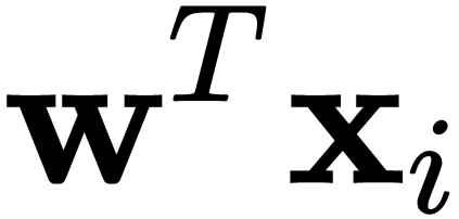
The trainable parameters of a neuron are w and b, and they are unknown. Thus, we can use training data to determine these parameters using some learning strategy. From the picture, x₁ multiplies w₁, then x₂ multiplies w₂, and b is multiplied by 1; all these products are added, which can be simplified as follows:

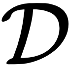
The activation function operates as a way to ensure the output is within the desired output range. Let's say that we want a simple linear activation, then the function z(.) is non-existing or can be bypassed, as follows:

This is usually the case when we want to solve a regression problem and the output data can have a range from -∞ to +∞. However, we may want to train the neuron to determine whether a vector x belongs to one of two classes, say -1 and +1. Then we would be better suited using a function called a sign activation:

Where the sign(.) function is denoted as follows:

There are many other activation functions, but we will introduce those later on. For now, we will briefly show one of the simplest learning algorithms, the perceptron learning algorithm (PLA).

The perceptron learning algorithm

The PLA begins from the assumption that you want to classify data, X, into two different groups, the positive group (+) and the negative group (-). It will find some w and b by training to predict the corresponding correct labels y. The PLA uses the sign( . ) function as the activation. Here are the steps that the PLA follows:

1. Initialize w to zeros, and iteration counter t = 0
2. While there are any incorrectly classified examples:

• Pick an incorrectly classified example, call it x^*, whose true label is y^*
• Update w as follows: w_t+1 = w_t + y^*x^*
• Increase iteration counter t++ and repeat

Notice that, for the PLA to work as we want, we have to make an adjustment. What we want is for to be implied in the expression . The only way this could work is if we set and . The previous rule seeks w, which implies the search for b.

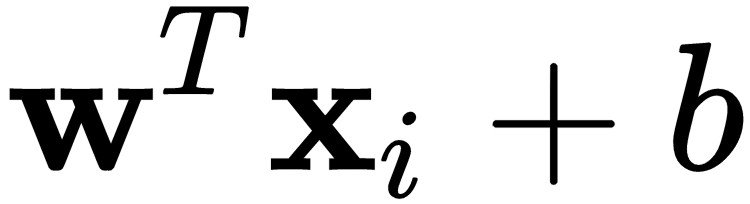
To illustrate the PLA, consider the case of the following linearly separable dataset:

This two-dimensional dataset was produced at random using Python tools that we will discuss later on. For now, it should be self-evident that you can draw a line between the two groups and divide them.

Following the steps outlined previously, the PLA can find a solution, that is, a separating line that satisfies the training data target outputs completely in only four iterations in this particular case. The plots after each update are depicted in the following plots with the corresponding line found at every update:

At iteration zero, all 100 points are misclassified, but after randomly choosing one misclassified point to make the first update, the new line only misses four points:

After the second update, the line only misses one data point:

Finally, after update number three, all data points are correctly classified. This is just to show that a simple learning algorithm can successfully learn from data. Also, the perceptron model led to much more complicated models such as a neural network. We will now introduce the concept of a shallow network and its basic complexities.

Shallow networks

A neural network consists of multiple networks connected in different layers. In contrast, a perceptron has only one neuron and its architecture consists of an input layer and an output layer. In neural networks, there are additional layers between the input and output layer, as shown in Figure 1.4, and they are known as hidden layers:

The example in the figure shows a neural network that has a hidden layer with eight neurons in it. The input size is 10-dimensional, and the output layer has four dimensions (four neurons). This intermediate layer can have as many neurons as your system can handle during training, but it is usually a good idea to keep things to a reasonable number of neurons.

Neural networks can solve more difficult problems than without a network, for example, with a single neural unit such as the perceptron. This must feel intuitive and must be easy to conceive. A neural network can solve problems including and beyond those that are linearly separable. For linearly separable problems, we can use both the perceptron model and a neural network. However, for more complex and non-linearly separable problems, the perceptron cannot offer a high-quality solution, while a neural network does.

For example, if we consider the sample two-class dataset and we bring the data groups closer together, the perceptron will fail to terminate with a solution and some other strategy can be used to stop it from going forever. Or, we can switch to a neural network and train it to find the best solution it can possibly find. Figure 1.5 shows an example of training a neural network with 100 neurons in the hidden layer over a two-class dataset that is not linearly separable:

This neural network has 100 neurons in the hidden layer. This was a choice done by experimentation and you will learn strategies on how to find such instances in further chapters. However, before we go any further, there are two new terms introduced that require further explanation: non-separable data and non-linear models, which are defined as follows:

• Non-separable data is such that there is no line that can separate groups of data (or classes) into two groups.
• Non-linear models, or solutions, are those that naturally and commonly occur when the best solution to a classification problem is not a line. For example, it can be some curve described by some polynomial of any degree greater than one. For an example, see Figure 1.5.

A non-linear model is usually what we will be working with throughout this book, and the reason is that this is most likely what you will encounter out there in the real world. Also, it is non-linear, in a way, because the problem is non-separable. To achieve this non-linear solution, the neural network model goes through the following mathematical operations.

The input-to-hidden layer

In a neural network, the input vector x is connected to a number of neurons through weights w for each neuron, which can be now thought of as a number of weight vectors forming a matrix W. The matrix W has as many columns as neurons as the layer has, and as many rows as the number of features (or dimensions) x has. Thus, the output of the hidden layer can be thought of as the following vector:

Where b is a vector of biases, whose elements correspond to one neural unit, and the size of h is proportional to the number of hidden units. For example, eight neurons in Figure 1.4, and 100 neurons in Figure 1.5. However, the activation function z(.) does not have to be the sign(.) function, in fact, it usually never is. Instead, most people use functions that are easily differentiable.

The hidden-to-hidden layer

In a neural network, we could have more than one single hidden layer, and we will work with this kind a lot in this book. In such case, the matrix W can be expressed as a three-dimensional matrix that will have as many elements in the third dimension and as many hidden layers as the network has. In the case of the i-th layer, we will refer to that matrix as W_i for convenience.

Therefore, we can refer to the output of the i-th hidden layer as follows:

For i = 2, 3, ..., k-1, where k is the total number of layers, and the case of h₁ is computed with the equation given for the first layer (see previous section), which uses x directly, and does not go all the way to the last layer, h_k, because that is computed as discussed next.

The hidden-to-output layer

The overall output of the network is the output at the last layer:

Here, the last activation function is usually different from the hidden layer activations. The activation function in the last layer (output) traditionally depends on the type of problem we are trying to solve. For example, if we want to solve a regression problem, we would use a linear function, or sigmoid activations for classification problems. We will discuss those later on. For now, it should be evident that the perceptron algorithm will no longer work in the training phase.

While the learning still has to be in terms of the mistakes the neural network makes, the adjustments cannot be in direct proportion to the data point that is incorrectly classified or predicted. The reason is that the neurons in the last layer are responsible for making the predictions, but they depend on a previous layer, and those may depend on more previous layers, and when making adjustments to W and b, the adjustment has to be made differently for each neuron.

One approach to do this is to apply gradient descent techniques on the neural network. There are many of these techniques and we will discuss the most popular of these in further chapters. In general, a gradient descent algorithm is one that uses the notion that, if you take the derivative of a function and that reaches a value of zero, then you have found the maximum (or minimum) value you can get for the set of parameters on which you are taking the derivatives. For the case of scalars, we call them derivatives, but for vectors or matrices (W, b), we call them gradients.

The function we can use is called a loss function.

We can define a loss function, for example, as follows:

This loss is known as the mean squared error (MSE); it is meant to measure how different the target output y is from the predicted output in the output layer h_k in terms of the square of its elements, and averaged. This is a good loss because it is differentiable and it is easy to compute.

A neural network such as this introduced a great number of possibilities, but relied heavily on a gradient descent technique for learning them called backpropagation (Hecht-Nielsen, R. 1992). Rather than explaining backpropagation here (we will reserve that for later), we rather have to remark that it changed the world of ML, but did not make much progress for a number of years because it had some practical limitations and the solutions to these paved the way for deep learning.

Deep networks

On March 27, 2019, an announcement was published by the ACM saying that three computer scientists were awarded the Nobel Prize in computing, that is, the ACM Turing Award, for their achievements in deep learning. Their names are Yoshua Bengio, Yann LeCun, and Geoffrey Hinton; all are very accomplished scientists. One of their major contributions was in the learning algorithm known as backpropagation.

In the official communication, the ACM wrote the following about Dr. Hinton and one of his seminal papers (Rumelhart, D. E. 1985):

Similarly, they wrote the following about Dr. LeCun's paper (LeCun, Y., et.al., 1998):

Dr. Hinton was able to show that there was a way to minimize a loss function in neural networks using biologically inspired algorithms such as the backward and forward adjustment of connections by modifying its importance for particular neurons. Usually, backpropagation is related to feed-forward neural networks, while backward-forward propagation is related to Restricted Boltzmann Machines (covered in Chapter 10, Restricted Boltzmann Machines).

A feed-forward neural network is one whose input is pipelined directly toward the output layer through intermediate layers that have no backward connections, as shown in Figure 1.4, and we will talk about these all the time in this book.

Backpropagation enabled people to train neural networks in a way that was never seen before; however, people had problems training neural networks on large datasets, and on larger (deeper) architectures. If you go ahead and look at neural network papers in the late '80s and early '90s, you will notice that architectures were small in size; networks usually had no more than two or three layers, and the number of neurons usually did not exceed the order of hundreds. These are (today) known as shallow neural networks.

The major problems were with convergence time for larger datasets, and convergence time for deeper architectures. Dr. LeCun's contributions were precisely in this area as he envisioned different ways to speed up the training process. Other advances such as vector (tensor) computations over graphics processing units (GPUs) increased training speeds dramatically.

Thus, over the last few years, we have seen the rise of deep learning, that is, the ability to train deeper neural networks, with more than three or four layers, in fact with tens and hundreds of layers. Further, we have a wide variety of architectures that can accomplish things that we were not able in the last decade.

The deep network shown in Figure 1.6 would have been impossible to train 30 years ago, and it is not that deep anyway:

Regardless of the future of DL, let us now discuss what makes DL so important today.

Today, we enjoy the benefits of algorithms and strategies that we did not have 20 or 30 years ago, which enable us to have amazing applications that are changing lives. Allow me to summarize some of the great and important things about deep learning today:

• Training in mini-batches: This strategy allows us today to have very large datasets and train a deep learning model little by little. In the past, we would have to load the entire dataset into memory, making it computationally impossible for some large datasets. Today, yes, it may take a little longer, but we at least can actually perform training on finite time.
• Novel activation functions: Rectified linear units (ReLUs), for example, are a relatively new kind of activation that solved many of the problems with large-scale training with backpropagation strategies. These new activations enable training algorithms to converge on deep architectures when, in the past, we would get stuck on non-converging training sessions that would end up having exploding or vanishing gradients.
• Novel neural network architectures: Convolutional or recurrent networks, for example, have been transforming the world by opening the possibilities of things we can do with neural networks. Convolutional networks are widely applied in computer vision applications or other areas in which the convolution operation is a natural thing to do, for example, multi-dimensional signal or audio analysis. Recurrent neural networks with memory are widely used to analyze sequences of text, thus enabling us to have networks that understand words, sentences, and paragraphs, and we can use them to translate between languages, and many more things.
• Interesting loss functions: These losses play an interesting role in deep learning because, in the past, we only used the same standard losses over and over again; losses such as the MSE. Today, we can minimize the MSE and, at the same time, minimize the norm of the weights or the output of some neurons, which leads to sparser weights and solutions that, in turn, make the produced model much more efficient when it is deployed into production.

• Novel strategies resembling biology: Things such as missing or dropping connections between neurons, rather than having them fully connected all the time, is more realistic, or comparable to biological neural network design. Also, dropping or removing neurons altogether is a new strategy that can push some neurons to excel when others are removed, learning richer representations, while at the same time reducing the computations during training and when deployed. The sharing of parameters between different and specialized neural networks also has proven to be interesting and effective today.
• Adversarial training: Making a neural network compete against another network whose sole purpose is to generate fraudulent, noisy, and confusing data points trying to make the network fail has proven to be an excellent strategy for networks to learn better from the data and be robust against noisy environments when deployed into production.

There are many other interesting facts and points that make deep learning an exciting area and justify the writing of this book. I hope you are as excited as we all are and begin reading this book knowing that we are going to code some of the most exciting and incredible neural networks of our time. Our ultimate purpose will be to make deep neural networks that can generalize.

This introductory chapter presented an overview of ML. It introduced the motivation behind ML and the terminology that is commonly used in the field. It also introduced deep learning and how it fits in the realm of artificial intelligence. At this point, you should feel confident that you know enough about what a neural network is to be curious about how big it can be. You should also feel very intrigued about the area of deep learning and all the new things that are coming out every week.

At this point, you must be a bit anxious to begin your deep learning coding journey; for that reason, the next logical step is to go to Chapter 2, Setup and Introduction to Deep Learning Frameworks. In this chapter, you will get ready for the action by setting up your system and making sure you have access to the resources you will need to be a successful deep learning practitioner. But before you go there, please try to quiz yourself with the following questions.

1. Can a perceptron and/or a neural network solve the problem of classifying data that is linearly separable?

Yes, both can.

2. Can a perceptron and/or a neural network solve the problem of classifying data that is non-separable?

Yes, both can. However, the perceptron will go on forever unless we specify a stopping condition such as a maximum number of iterations (updates), or stopping if the number of misclassified points does not decrease after a number of iterations.

3. What are the changes in the ML filed that have enabled us to have deep learning today?

(A) backpropagation algorithms, batch training, ReLUs, and so on;

(B) computing power, GPUs, cloud, and so on.

4. Why is generalization a good thing?

Because deep neural networks are most useful when they can function as expected when they are given data that they have not seen before, that is, data on which they have not been trained.

• Hecht-Nielsen, R. (1992). Theory of the backpropagation neural network. In Neural networks for perception (pp. 65-93). Academic Press.
• Kane, F. (2017). Hands-On Data Science and Python ML. Packt Publishing Ltd.
• LeCun, Y., Bottou, L., Orr, G., and Muller, K. (1998). Efficient backprop in neural networks: Tricks of the trade (Orr, G. and Müller, K., eds.). Lecture Notes in Computer Science, 1524(98), 111.
• Ojeda, T., Murphy, S. P., Bengfort, B., and Dasgupta, A. (2014). Practical Data Science Cookbook. Packt Publishing Ltd.

• Rosenblatt, F. (1958). The perceptron: a probabilistic model for information storage and organization in the brain. Psychological Review, 65(6), 386.
• Rumelhart, D. E., Hinton, G. E., and Williams, R. J. (1985). Learning internal representations by error propagation (No. ICS-8506). California Univ San Diego La Jolla Inst for Cognitive Science.