


 Download code from GitHub
First Steps
Whether you are an eager learner of data science or a well-grounded data science practitioner, you can take advantage of this essential introduction to Python for data science. You can use it to the fullest if you already have at least some previous experience in basic coding, in writing general-purpose computer programs in Python, or in some other data-analysis-specific language such as MATLAB or R.
This book will delve directly into Python for data science, providing you with a straight and fast route to solving various data science problems using Python and its powerful data analysis and machine learning packages. The code examples that are provided in this book don't require you to be a master of Python. However, they will assume that you at least know the basics of Python scripting, including data structures such as lists and dictionaries, and the workings of class objects. If you don't feel confident about these subjects or have minimal knowledge of the Python language, before reading this book, we suggest that you take an online tutorial. There are good online tutorials that you may take, such as the one offered by the Code Academy course at https://www.codecademy.com/learn/learn-python, the one by Google's Python class at https://developers.google.com/edu/python/, or even the Whirlwind tour of Python by Jake Vanderplas (https://github.com/jakevdp/WhirlwindTourOfPython). All the courses are free, and, in a matter of a few hours of study, they should provide you with all the building blocks that will ensure you enjoy this book to the fullest. In order to provide an integration of the two aforementioned free courses, we have also prepared a tutorial of our own, which can be found in the appendix of this book.
In any case, don't be intimidated by our starting requirements; mastering Python enough for data science applications isn't as arduous as you may think. It's just that we have to assume some basic knowledge on the reader's part because our intention is to go straight to the point of doing data science without having to explain too much about the general aspects of the Python language that we will be using.
Are you ready, then? Let's get started!
In this short introductory chapter, we will work through the basics to set off in full swing and go through the following topics:
- How to set up a Python data science toolbox
- Using Jupyter
- An overview of the data that we are going to study in this book
Introducing data science and Python
Data science is a relatively new knowledge domain, though its core components have been studied and researched for many years by the computer science community. Its components include linear algebra, statistical modeling, visualization, computational linguistics, graph analysis, machine learning, business intelligence, and data storage and retrieval.
Data science is a new domain, and you have to take into consideration that, currently, its frontiers are still somewhat blurred and dynamic. Since data science is made of various constituent sets of disciplines, please also keep in mind that there are different profiles of data scientists depending on their competencies and areas of expertise (for instance, you may read the illustrative There’s More Than One Kind of Data Scientist by Harlan D Harris at radar.oreilly.com/2013/06/theres-more-than-one-kind-of-data-scientist.html, or delve into the discussion about type A or B data scientists and other interesting taxonomies at https://stats.stackexchange.com/questions/195034/what-is-a-data-scientist).
In such a situation, what can be the best tool of the trade that you can learn and effectively use in your career as a data scientist? We believe that the best tool is Python, and we intend to provide you with all the essential information that you will need for a quick start.
In addition, other programming languages such as R and MATLAB provide data scientists with specialized tools to solve specific problems in statistical analysis and matrix manipulation in data science. However, only Python really completes your data scientist skill set with all the key techniques in a scalable and effective way. This multipurpose language is suitable for both development and production alike; it can handle small- to large-scale data problems and it is easy to learn and grasp, no matter what your background or experience is.
Created in 1991 as a general-purpose, interpreted, and object-oriented language, Python has slowly and steadily conquered the scientific community and grown into a mature ecosystem of specialized packages for data processing and analysis. It allows you to have uncountable and fast experimentations, easy theory development, and prompt deployment of scientific applications.
At present, the core Python characteristics that render it an indispensable data science tool are as follows:
- It offers a large, mature system of packages for data analysis and machine learning. It guarantees that you will get all that you may need in the course of a data analysis, and sometimes even more.
- Python can easily integrate different tools and offers a truly unifying ground for different languages, data strategies, and learning algorithms that can be fitted together easily and which can concretely help data scientists forge powerful solutions. There are packages that allow you to call code in other languages (in Java, C, Fortran, R, or Julia), outsourcing some of the computations to them and improving your script performance.
- It is very versatile. No matter what your programming background or style is (object-oriented, procedural, or even functional), you will enjoy programming with Python.
- It is cross-platform; your solutions will work perfectly and smoothly on Windows, Linux, and macOS systems. You won't have to worry all that much about portability.
- Although interpreted, it is undoubtedly fast compared to other mainstream data analysis languages such as R and MATLAB (though it is not comparable to C, Java, and the newly emerged Julia language). Moreover, there are also static compilers such as Cython or just-in-time compilers such as PyPy that can transform Python code into C for higher performance.
- It can work with large in-memory data because of its minimal memory footprint and excellent memory management. The memory garbage collector will often save the day when you load, transform, dice, slice, save, or discard data using various iterations and reiterations of data wrangling.
- It is very simple to learn and use. After you grasp the basics, there's no better way to learn more than by immediately starting with the coding.
- Moreover, the number of data scientists using Python is continuously growing: new packages and improvements have been released by the community every day, making the Python ecosystem an increasingly prolific and rich language for data science.
Installing Python
First, let's proceed and introduce all the settings you need in order to create a fully working data science environment to test the examples and experiment with the code that we are going to provide you with.
Python is an open source, object-oriented, and cross-platform programming language. Compared to some of its direct competitors (for instance, C++ or Java), Python is very concise. It allows you to build a working software prototype in a very short time, and yet it has become the most used language in the data scientist's toolbox not just because of that. It is also a general-purpose language, and it is very flexible due to a variety of available packages that solve a wide spectrum of problems and necessities.
Python 2 or Python 3?
There are two main branches of Python: 2.7.x and 3.x. At the time of the revision of this third edition of the book, the Python foundation (www.python.org/) is offering downloads for Python Version 2.7.15 (release date January 5, 2018) and 3.6.5 (release date January 3, 2018). Although the Python 3 version is the newest, the older Python 2 has still been in use in both scientific (20% adoption) and commercial (30% adoption) areas in 2017, as depicted in detail by this survey by JetBrains: https://www.jetbrains.com/research/python-developers-survey-2017. If you are still using Python 2, the situation could turn quite problematic soon, because in just one year's time Python 2 will be retired and maintenance will be ceased (pythonclock.org/ will provide you with the countdown, but for an official statement about this, just read https://www.python.org/dev/peps/pep-0373/), and there are really only a handful of libraries still incompatible between the two versions (py3readiness.org/) that do not give enough reasons to stay with the older version.
In addition to all these reasons, there is no immediate backward compatibility between Python 3 and 2. In fact, if you try to run some code developed for Python 2 with a Python 3 interpreter, it may not work. Major changes have been made to the newest version, and that has affected past compatibility. Some data scientists, having built most of their work on Python 2 and its packages, are reluctant to switch to the new version.
In this third edition of the book, we will continue to address the larger audience of data scientists, data analysts, and developers, who do not have such a strong legacy with Python 2. Consequently, we will continue working with Python 3, and we suggest using a version such as the most recently available Python 3.6. After all, Python 3 is the present and the future of Python. It is the only version that will be further developed and improved by the Python foundation, and it will be the default version of the future on many operating systems.
Anyway, if you are currently working with version 2 and you prefer to keep on working with it, you can still use this book and all of its examples. In fact, for the most part, our code will simply work on Python 2 after having the code itself preceded by these imports:
from __future__ import (absolute_import, division,
                        print_function, unicode_literals)
from builtins import *
from future import standard_library
standard_library.install_aliases()
As described in the Python-future website (python-future.org), these imports will help convert several Python 3-only constructs to a form that's compatible with both Python 3 and Python 2 (and in any case, most Python 3 code should just simply work on Python 2, even without the aforementioned imports).
In order to run the upward commands successfully, if the future package is not already available on your system, you should install it (version >= 0.15.2) by using the following command, which is to be executed from a shell:
$> pip install -U future
If you're interested in understanding the differences between Python 2 and Python 3 further, we recommend reading the wiki page offered by the Python foundation itself: https://wiki.python.org/moin/Python2orPython3.
Step-by-step installation
Novice data scientists who have never used Python (who likely don't have the language readily installed on their machines) need to first download the installer from the main website of the project, www.python.org/downloads/, and then install it on their local machine.
This being a multiplatform programming language, you'll find installers for machines that either run on Windows or Unix-like operating systems.
Remember that some of the latest versions of most Linux distributions (such as CentOS, Fedora, Red Hat Enterprise, and Ubuntu) have Python 2 packaged in the repository. In such a case, and in the case that you already have a Python version on your computer (since our examples run on Python 3), you first have to check what version you are exactly running. To do such a check, just follow these instructions:
- Open a python shell, type python in the terminal, or click on any Python icon you find on your system.
- Then, after starting Python, to test the installation, run the following code in the Python interactive shell or REPL:
>>> import sys
>>> print (sys.version_info)
- If you can read that your Python version has the major=2 attribute, it means that you are running a Python 2 instance. Otherwise, if the attribute is valued 3, or if the print statement reports back to you something like v3.x.x (for instance, v3.5.1), you are running the right version of Python, and you are ready to move forward.
To clarify the operations we have just mentioned, when a command is given in the terminal command line, we prefix the command with $>. Otherwise, if it's for the Python REPL, it's preceded by >>>.
Installing the necessary packages
Python won't come bundled with everything you need unless you take a specific pre-made distribution. Therefore, to install the packages you need, you can use either pip or easy_install. Both of these two tools run in the command line and make the process of installation, upgrading, and removing Python packages a breeze. To check which tools have been installed on your local machine, run the following command:
$> pip
Alternatively, you can also run the following command:
$> easy_install
If both of these commands end up with an error, you need to install any one of them. We recommend that you use pip because it is thought of as an improvement over easy_install. Moreover, easy_install is going to be dropped in the future and pip has important advantages over it. It is preferable to install everything using pip because of the following:
- It is the preferred package manager for Python 3. Starting with Python 2.7.9 and Python 3.4, it is included by default with the Python binary installers
- It provides an uninstall functionality
- It rolls back and leaves your system clear if, for whatever reason, the package's installation fails
The most recent versions of Python should already have pip installed by default. Therefore, you may have it already installed on your system. If not, the safest way is to download the get-pi.py script from https://bootstrap.pypa.io/get-pip.py and then run it by using the following:
$> python get-pip.py
The script will also install the setup tool from pypi.org/project/setuptools, which also contains easy_install.
You're now ready to install the packages you need in order to run the examples provided in this book. To install the < package-name > generic package, you just need to run the following command:
$> pip install < package-name >
Alternatively, you can run the following command:
$> easy_install < package-name >
Note that, in some systems, pip might be named as pip3 and easy_install as easy_install-3 to stress the fact that both operate on packages for Python 3. If you're unsure, check the version of Python that pip is operating on with:
$> pip -V
For easy_install, the command is slightly different:
$> easy_install --version
After this, the <pk> package and all its dependencies will be downloaded and installed. If you're not certain whether a library has been installed or not, just try to import a module inside it. If the Python interpreter raises an ImportError error, it can be concluded that the package has not been installed.
This is what happens when the NumPy library has been installed:
>>> import numpy
This is what happens if it's not installed:
>>> import numpy

    Traceback (most recent call last):
    File "<stdin>", line 1, in <module>
    ImportError: No module named numpy
In the latter case, you'll need to first install it through pip or easy_install.
Finally, to search and browse the Python packages available for Python, look at pypi.org.
Package upgrades
More often than not, you will find yourself in a situation where you have to upgrade a package because either the new version is required by a dependency or it has additional features that you would like to use. First, check the version of the library you have installed by glancing at the __version__ attribute, as shown in the following example, numpy:
>>> import numpy
>>> numpy.__version__ # 2 underscores before and after
    '1.11.0'
Now, if you want to update it to a newer release, say the 1.12.1 version, you can run the following command from the command line:
$> pip install -U numpy==1.12.1
Alternatively, you can use the following command:
$> easy_install --upgrade numpy==1.12.1
Finally, if you're interested in upgrading it to the latest available version, simply run the following command:
$> pip install -U numpy
You can alternatively run the following command:
$> easy_install --upgrade numpy
Scientific distributions
As you've read so far, creating a working environment is a time-consuming operation for a data scientist. You first need to install Python, and then, one by one, you can install all the libraries that you will need (sometimes, the installation procedures may not go as smoothly as you'd hoped for earlier).
If you want to save time and effort and want to ensure that you have a fully working Python environment that is ready to use, you can just download, install, and use the scientific Python distribution. Apart from Python, they also include a variety of preinstalled packages, and sometimes, they even have additional tools and an IDE. A few of them are very well-known among data scientists, and in the sections that follow, you will find some of the key features of each of these packages.
We suggest that you first promptly download and install a scientific distribution, such as Anaconda (which is the most complete one), and after practicing the examples in this book, decide whether or not to fully uninstall the distribution and set up Python alone, which can be accompanied by just the packages you need for your projects.
Anaconda
Anaconda (https://www.anaconda.com/download/) is a Python distribution offered by Continuum Analytics that includes nearly 200 packages, which comprises NumPy, SciPy, pandas, Jupyter, Matplotlib, Scikit-learn, and NLTK. It's a cross-platform distribution (Windows, Linux, and macOS) that can be installed on machines with other existing Python distributions and versions. Its base version is free; instead, add-ons that contain advanced features are charged separately. Anaconda introduces conda, a binary package manager, as a command-line tool to manage your package installations.
As stated on the website, Anaconda's goal is to provide enterprise-ready Python distribution for large-scale processing, predictive analytics, and scientific computing.
Leveraging conda to install packages
If you've decided to install an Anaconda distribution, you can take advantage of the conda binary installer we mentioned previously. conda is an open source package management system, and consequently, it can be installed separately from an Anaconda distribution. The core difference from pip is that conda can be used to install any package (not just Python's ones) in a conda environment (that is, an environment where you have installed conda and you are using it for providing packages). There are many advantages in using conda over pip, as described by Jack VanderPlas in this famous blog post of his: jakevdp.github.io/blog/2016/08/25/conda-myths-and-misconceptions.
You can test immediately whether conda is available on your system. Open a shell and digit the following:
$> conda -V
If conda is available, your version will appear; otherwise, an error will be reported. If conda is not available, you can quickly install it on your system by going to http://conda.pydata.org/miniconda.html and installing the Miniconda software that's suitable for your computer. Miniconda is a minimal installation that only includes conda and its dependencies.
Conda can help you manage two tasks: installing packages and creating virtual environments. In this paragraph, we will explore how conda can help you easily install most of the packages you may need in your data science projects.
Before starting, please check that you have the latest version of conda at hand:
$> conda update conda
Now you can install any package you need. To install the <package-name> generic package, you just need to run the following command:
$> conda install <package-name>
You can also install a particular version of the package just by pointing it out:
$> conda install <package-name>=1.11.0
Similarly, you can install multiple packages at once by listing all their names:
$> conda install <package-name-1> <package-name-2>
If you just need to update a package that you previously installed, you can keep on using conda:
$> conda update <package-name>
You can update all the available packages simply by using the --all argument:
$> conda update --all
Finally, conda can also uninstall packages for you:
$> conda remove <package-name>
If you would like to know more about conda, you can read its documentation at http://conda.pydata.org/docs/index.html. In summary, as its main advantage, it handles binaries even better than easy_install (by always providing a successful installation on Windows without any need to compile the packages from source) but without its problems and limitations. With the use of conda, packages are easy to install (and installation is always successful), update, and even uninstall. On the other hand, conda cannot install directly from a git server (so it cannot access the latest version of many packages under development), and it doesn't cover all the packages available on PyPI like pip itself.
Enthought Canopy
Enthought Canopy (https://www.enthought.com/products/canopy/) is a Python distribution by Enthought Inc. It includes more than 200 preinstalled packages, such as NumPy, SciPy, Matplotlib, Jupyter, and pandas. This distribution is targeted at engineers, data scientists, quantitative and data analysts, and enterprises. Its base version is free (which is named Canopy Express), but if you need advanced features, you have to buy a front version. It's a multi-platform distribution, and its command-line installation tool is canopy_cli.
WinPython
WinPython (http://winpython.github.io/) is a free, open-source Python distribution that's maintained by the community. It is designed for scientists and includes many packages such as NumPy, SciPy, Matplotlib, and Jupyter. It also includes Spyder as an IDE. It is free and portable. You can put WinPython into any directory, or even into a USB flash drive, and at the same time maintain multiple copies and versions of it on your system. It only works on Microsoft Windows, and its command-line tool is the WinPython Package Manager (WPPM).
Explaining virtual environments
No matter whether you have chosen to install a standalone Python or instead used a scientific distribution, you may have noticed that you are actually bound on your system to the Python version you have installed. The only exception, for Windows users, is to use a WinPython distribution, since it is a portable installation and you can have as many different installations as you need.
A simple solution to breaking free of such a limitation is to use virtualenv, which is a tool for creating isolated Python environments. That means, by using different Python environments, you can easily achieve the following things:
- Testing any new package installation or doing experimentation on your Python environment without any fear of breaking anything in an irreparable way. In this case, you need a version of Python that acts as a sandbox.
- Having at hand multiple Python versions (both Python 2 and Python 3), geared with different versions of installed packages. This can help you in dealing with different versions of Python for different purposes (for instance, some of the packages we are going to present on Windows OS only work when using Python 3.4, which is not the latest release).
- Taking a replicable snapshot of your Python environment easily and having your data science prototypes work smoothly on any other computer or in production. In this case, your main concern is the immutability and replicability of your working environment.
You can find documentation about virtualenv at http://virtualenv.readthedocs.io/en/stable/, though we are going to provide you with all the directions you need to start using it immediately. In order to take advantage of virtualenv, you first have to install it on your system:
$> pip install virtualenv
After the installation completes, you can start building your virtual environments. Before proceeding, you have to make a few decisions:
- If you have more versions of Python installed on your system, you have to decide which version to pick up. Otherwise, virtualenv will take the Python version that was used when virtualenv was installed on your system. In order to set a different Python version, you have to digit the argument -p followed by the version of Python you want, or insert the path of the Python executable to be used (for instance, by using -p python2.7, or by just pointing to a Python executable such as -p c:Anaconda2python.exe).
- With virtualenv, when required to install a certain package, it will install it from scratch, even if it is already available at a system level (on the python directory you created the virtual environment from). This default behavior makes sense because it allows you to create a completely separated empty environment. In order to save disk space and limit the time of installation of all the packages, you may instead decide to take advantage of already available packages on your system by using the argument --system-site-packages.
- You may want to be able to later move around your virtual environment across Python installations, even among different machines. Therefore, you may want to make the functionality of all of the environment's scripts relative to the path it is placed in by using the argument --relocatable.
After deciding on the Python version you wish to use, linking to existing global packages, and the virtual environment being relocatable or not, in order to start, you just need to launch the command from a shell. Declare the name you would like to assign to your new environment:
$> virtualenv clone
virtualenv will just create a new directory using the name you provided, in the path from which you actually launched the command. To start using it, you can just enter the directory and digit activate:
$> cd clone
$> activate
At this point, you can start working on your separated Python environment, installing packages, and working with code.
If you need to install multiple packages at once, you may need some special function from pip, pip freeze, which will enlist all the packages (and their versions) you have installed on your system. You can record the entire list in a text file by using the following command:
$> pip freeze > requirements.txt
After saving the list in a text file, just take it into your virtual environment and install all the packages in a breeze with a single command:
$> pip install -r requirements.txt
Each package will be installed according to the order in the list (packages are listed in a case-insensitive sorted order). If a package requires other packages that are later in the list, that's not a big deal because pip automatically manages such situations. So, if your package requires NumPy and NumPy is not yet installed, pip will install it first.
When you've finished installing packages and using your environment for scripting and experimenting, in order to return to your system defaults, just issue the following command:
$> deactivate
If you want to remove the virtual environment completely, after deactivating and getting out of the environment's directory, you just have to get rid of the environment's directory itself by performing a recursive deletion. For instance, on Windows, you just do the following:
$> rd /s /q clone
On Linux and macOS, the command will be as follows:
$> rm -r -f clone
Conda for managing environments
If you have installed the Anaconda distribution, or you have tried conda by using a Miniconda installation, you can also take advantage of the conda command to run virtual environments as an alternative to virtualenv. Let's see how to use conda for that in practice. We can check what environments we have available like this:
>$ conda info -e
This command will report to you what environments you can use on your system based on conda. Most likely, your only environment will be root, pointing to your Anaconda distribution folder.
As an example, we can create an environment based on Python Version 3.6, having all the necessary Anaconda-packaged libraries installed. This makes sense, for instance, when installing a particular set of packages for a data science project. In order to create such an environment, just perform the following:
$> conda create -n python36 python=3.6 anaconda
The preceding command asks for a particular Python version, 3.6, and requires the installation of all packages that are available on the Anaconda distribution (the argument anaconda). It names the environment as python36 using the argument -n. The complete installation should take a while, given a large number of packages in the Anaconda installation. After having completed all of the installations, you can activate the environment:
$> activate python36
If you need to install additional packages to your environment when activated, you just use the following:
$> conda install -n python36 <package-name1> <package-name2>
That is, you make the list of the required packages follow the name of your environment. Naturally, you can also use pip install, as you would do in a virtualenv environment.
You can also use a file instead of listing all the packages by name yourself. You can create a list in an environment using the list argument and pipe the output to a file:
$> conda list -e > requirements.txt
Then, in your target environment, you can install the entire list by using the following:
$> conda install --file requirements.txt
You can even create an environment, based on a requirements list:
$> conda create -n python36 python=3.6 --file requirements.txt
Finally, after having used the environment, to close the session, you simply use the following command:
$> deactivate
Contrary to virtualenv, there is a specialized argument in order to completely remove an environment from your system:
$> conda remove -n python36 --all
A glance at the essential packages
We mentioned previously that the two most relevant characteristics of Python are its ability to integrate with other languages and its mature package system, which is well embodied by PyPI (the Python Package Index: pypi.org), a common repository for the majority of Python open source packages that are constantly maintained and updated.
The packages that we are now going to introduce are strongly analytical and they will constitute a complete data science toolbox. All of the packages are made up of extensively tested and highly optimized functions for both memory usage and performance, ready to achieve any scripting operation with successful execution. A walkthrough on how to install them is provided in the following section.
Partially inspired by similar tools present in R and MATLAB environments, we will explore how a few selected Python commands can allow you to efficiently handle data and then explore, transform, experiment, and learn from the same without having to write too much code or reinvent the wheel.
NumPy
NumPy, which is Travis Oliphant's creation, is the true analytical workhorse of the Python language. It provides the user with multidimensional arrays, along with a large set of functions to operate a multiplicity of mathematical operations on these arrays. Arrays are blocks of data that are arranged along multiple dimensions, which implement mathematical vectors and matrices. Characterized by optimal memory allocation, arrays are useful—not just for storing data, but also for fast matrix operations (vectorization), which are indispensable when you wish to solve ad hoc data science problems:
- Website: http://www.numpy.org/
- Version at the time of print: 1.12.1
- Suggested install command: pip install numpy
As a convention largely adopted by the Python community, when importing NumPy, it is suggested that you alias it as np:
import numpy as np
We will be doing this throughout the course of this book.
SciPy
An original project by Travis Oliphant, Pearu Peterson, and Eric Jones, SciPy completes NumPy's functionalities, which offers a larger variety of scientific algorithms for linear algebra, sparse matrices, signal and image processing, optimization, fast Fourier transformation, and much more:
- Website: http://www.scipy.org/
- Version at time of print: 1.1.0
- Suggested install command: pip install scipy
pandas
The pandas package deals with everything that NumPy and SciPy cannot do. Thanks to its specific data structures, namely DataFrames and Series, pandas allows you to handle complex tables of data of different types (which is something that NumPy's arrays cannot do) and time series. Thanks to Wes McKinney's creation, you will be able to easily and smoothly load data from a variety of sources. You can then slice, dice, handle missing elements, add, rename, aggregate, reshape, and finally visualize your data at will:
- Website: http://pandas.pydata.org/
- Version at the time of print: 0.23.1
- Suggested install command: pip install pandas
Conventionally, the pandas package is imported as pd:
import pandas as pd
pandas-profiling
This is a GitHub project that easily allows you to create a report from a pandas DataFrame. The package will present the following measures in an interactive HTML report, which is used to evaluate the data at hand for a data science project:
- Essentials, such as type, unique values, and missing values
- Quantile statistics, such as minimum value, Q1, median, Q3, maximum, range, and interquartile range
- Descriptive statistics such as mean, mode, standard deviation, sum, median absolute deviation, the coefficient of variation, kurtosis, and skewness
- Most frequent values
- Histograms
- Correlations highlighting highly correlated variables, and Spearman and Pearson matrixes
Here is all the information about this package:
- Website: https://github.com/pandas-profiling/pandas-profiling
- Version at the time of print: 1.4.1
- Suggested install command: pip install pandas-profiling
Scikit-learn
Started as part of SciKits (SciPy Toolkits), Scikit-learn is the core of data science operations in Python. It offers all that you may need in terms of data preprocessing, supervised and unsupervised learning, model selection, validation, and error metrics. Expect us to talk at length about this package throughout this book. Scikit-learn started in 2007 as a Google Summer of Code project by David Cournapeau. Since 2013, it has been taken over by the researchers at INRIA ( Institut national de recherche en informatique et en automatique, that is the French Institute for Research in Computer Science and Automation):
- Website: http://Scikit-learn.org/stable
- Version at the time of print: 0.19.1
- Suggested install command: pip install Scikit-learn
Jupyter
A scientific approach requires the fast experimentation of different hypotheses in a reproducible fashion. Initially named IPython and limited to working only with the Python language, Jupyter was created by Fernando Perez in order to address the need for an interactive Python command shell (which is based on shell, web browser, and the application interface), with graphical integration, customizable commands, rich history (in the JSON format), and computational parallelism for an enhanced performance. Jupyter is our favored choice throughout this book; it is used to clearly and effectively illustrate operations with scripts and data, and the consequent results:
- Website: http://jupyter.org/
- Version at the time of print: 4.4.0 (ipykernel = 4.8.2)
- Suggested install command: pip install jupyter
JupyterLab
JupyterLab is the next user interface for the Jupyter project, which is currently in beta. It is an environment devised for interactive and reproducible computing which will offer all the usual notebook, terminal, text editor, file browser, rich outputs, and so on arranged in a more flexible and powerful user interface. JupyterLab will eventually replace the classic Jupyter Notebook after JupyterLab reaches Version 1.0. Therefore, we intend to introduce this package now in order to make you aware of it and of its functionalities:
- Website: https://github.com/jupyterlab/jupyterlab
- Version at the time of print: 0.32.0
- Suggested install command: pip install jupyterlab
Matplotlib
Originally developed by John Hunter, matplotlib is a library that contains all the building blocks that are required to create quality plots from arrays and to visualize them interactively.
You can find all the MATLAB-like plotting frameworks inside the PyLab module:
- Website: http://matplotlib.org/
- Version at the time of print: 2.2.2
- Suggested install command: pip install matplotlib
You can simply import what you need for your visualization purposes with the following command:
import matplotlib.pyplot as plt
Seaborn
Working out beautiful graphics using matplotlib can be really time-consuming, for this reason, Michael Waskom (http://www.cns.nyu.edu/~mwaskom/) developed Seaborn, a high-level visualization package based on matplotlib and integrated with pandas data structures (such as Series and DataFrames) capable to produce informative and beautiful statistical visualizations.
- Website: http://seaborn.pydata.org/
- Version at the time of print: 0.9.0
- Suggested install command: pip install seaborn
You can simply import what you need for your visualization purposes with the following command:
import seaborn as sns
Statsmodels
Previously a part of SciKits, statsmodels was thought to be a complement to SciPy's statistical functions. It features generalized linear models, discrete choice models, time series analysis, and a series of descriptive statistics, as well as parametric and non-parametric tests:
- Website: http://statsmodels.sourceforge.net/
- Version at the time of print: 0.9.0
- Suggested install command: pip install statsmodels
Beautiful Soup
Beautiful Soup, a creation of Leonard Richardson, is a great tool to scrap out data from HTML and XML files that are retrieved from the internet. It works incredibly well, even in the case of tag soups (hence the name), which are collections of malformed, contradictory, and incorrect tags. After choosing your parser (the HTML parser included in Python's standard library works fine), thanks to Beautiful Soup, you can navigate through the objects in the page and extract text, tables, and any other information that you may find useful:
- Website: http://www.crummy.com/software/BeautifulSoup
- Version at the time of print: 4.6.0
- Suggested install command: pip install beautifulsoup4
NetworkX
Developed by the Los Alamos National Laboratory, NetworkX is a package specialized in the creation, manipulation, analysis, and graphical representation of real-life network data (it can easily operate with graphs made up of a million nodes and edges). Besides specialized data structures for graphs and fine visualization methods (2D and 3D), it provides the user with many standard graph measures and algorithms, such as the shortest path, centrality, components, communities, clustering, and PageRank. We will mainly use this package in Chapter 6, Social Network Analysis:
- Website: http://networkx.github.io/
- Version at the time of print: 2.1
- Suggested install command: pip install networkx
Conventionally, NetworkX is imported as nx:
import networkx as nx
NLTK
The Natural Language Toolkit (NLTK) provides access to corpora and lexical resources, and to a complete suite of functions for Natural Language Processing (NLP), ranging from tokenizers to part-of-speech taggers and from tree models to named-entity recognition. Initially, Steven Bird and Edward Loper created the package as an NLP teaching infrastructure for their course at the University of Pennsylvania. Now it is a fantastic tool that you can use to prototype and build NLP systems:
- Website: http://www.nltk.org/
- Version at the time of print: 3.3
- Suggested install command: pip install nltk
Gensim
Gensim, programmed by Radim Řehůřek, is an open source package that is suitable for the analysis of large textual collections with the help of parallel distributable online algorithms. Among advanced functionalities, it implements Latent Semantic Analysis (LSA), topic modeling by Latent Dirichlet Allocation (LDA), and Google's word2vec, a powerful algorithm that transforms text into vector features that can be used in supervised and unsupervised machine learning:
- Website: http://radimrehurek.com/gensim/
- Version at the time of print: 3.4.0
- Suggested install command: pip install gensim
PyPy
PyPy is not a package; it is an alternative implementation of Python 3.5.3 that supports most of the commonly used Python standard packages (unfortunately, NumPy is currently not fully supported). As an advantage, it offers enhanced speed and memory handling. Thus, it is very useful for heavy-duty operations on large chunks of data, and it should be part of your big data handling strategies:
- Website: http://pypy.org/
- Version at time of print: 6.0
- Download page: http://pypy.org/download.html
XGBoost
XGBoost is a scalable, portable, and distributed gradient boosting library (a tree ensemble machine learning algorithm). Initially created by Tianqi Chen from Washington University, it has been enriched by a Python wrapper by Bing Xu and an R interface by Tong He (you can read the story behind XGBoost directly from its principal creator at http://homes.cs.washington.edu/~tqchen/2016/03/10/story-and-lessons-behind-the-evolution-of-xgboost.html). XGBoost is available for Python, R, Java, Scala, Julia, and C++, and it can work on a single machine (leveraging multithreading) in both Hadoop and Spark clusters:
- Website: https://xgboost.readthedocs.io/en/latest/
- Version at the time of print: 0.80
- Download page: https://github.com/dmlc/xgboost
Detailed instructions for installing XGBoost on your system can be found at https://github.com/dmlc/xgboost/blob/master/doc/build.md.
The installation of XGBoost on both Linux and macOS is quite straightforward, whereas it is a little bit trickier for Windows users, though the recent release of a pre-built binary wheel for Python has made the procedure a piece of cake for everyone. You simply have to type this on your shell:
$> pip install xgboost
If you want to install XGBoost from scratch because you need the most recent bug fixes or GPU support, you need to first build the shared library from C++ (libxgboost.so for Linux/macOS and xgboost.dll for Windows) and then install the Python package. On a Linux/macOS system, you just have to build the executable by the make command, but on Windows, things are a little bit more tricky.
Generally, refer to https://xgboost.readthedocs.io/en/latest/build.html#, which provides the most recent instructions for building from scratch. For a quick reference, here, we are going to provide specific installation steps to get XGBoost working on Windows:
- First, download and install Git for Windows, (https://git-for-windows.github.io/).
- Then, you need a MINGW compiler present on your system. You can download it from http://www.mingw.org/ or http://tdm-gcc.tdragon.net/, according to the characteristics of your system.
- From the command line, execute the following:
$> git clone --recursive https://github.com/dmlc/xgboost
$> cd xgboost
$> git submodule init
$> git submodule update
- Then, always from the command line, copy the configuration for 64-byte systems to be the default one:
$> copy make\mingw64.mk config.mk
- Alternatively, you just copy the plain 32-byte version:
$> copy make\mingw.mk config.mk
- After copying the configuration file, you can run the compiler, setting it to use four threads in order to speed up the compiling procedure:
$> mingw32-make -j4
- In MinGW, the make command comes with the name mingw32-make. If you are using a different compiler, the previous command may not work. If so, you can simply try this:
$> make -j4
- Finally, if the compiler completes its work without errors, you can install the package in your Python by using the following:
$> cd python-package
$> python setup.py install
You just need to find the location on your computer of MinGW's binaries (in our case, it was in C:\mingw-w64\mingw64\bin; just modify the following code and put yours) and place the following code snippet before importing XGBoost:
import os
mingw_path = 'C:\mingw-w64\mingw64\bin'
os.environ['PATH']=mingw_path + ';' + os.environ['PATH']
import xgboost as xgb
LightGBM
LightGBM is a gradient boosting framework that was developed by Microsoft that uses the tree-based learning algorithm in a different fashion than other GBMs, favoring exploration of more promising leaves (leaf-wise) instead of developing level-wise.
In graph terminology, LightGBM is pursuing a depth-first search strategy than a breadth-first search one.
It has been designed to be distributed (Parallel and GPU learning supported), and its unique approach really achieves faster training speed with lower memory usage (thus allowing for the handling of the larger scale of data):
- Website: https://github.com/Microsoft/LightGBM
- Version at the time of print: 2.1.0
The installation of XGBoost requires some more actions on your side than usual Python packages. If you are operating on a Windows system, open a shell and issue the following commands:
$> git clone --recursive https://github.com/Microsoft/LightGBM
$> cd LightGBM
$> mkdir build
$> cd build
$> cmake -G "MinGW Makefiles" ..
$> mingw32-make.exe -j4
If you are instead operating on a Linux system, you just need to digit on a shell:
$> git clone --recursive https://github.com/Microsoft/LightGBM
$> cd LightGBM
$> mkdir build
$> cd build
$> cmake ..
$> make -j4
After you have completed compiling the package, no matter whether you are on Windows or Linux, you just import it on your Python command line:
import lightgbm as lgbm
CatBoost
Developed by Yandex researchers and engineers, CatBoost (which stands for categorical boosting) is a gradient boosting algorithm, based on decision trees, which is optimized in handling categorical features without much preprocessing (non-numeric features expressing a quality, such as a color, a brand, or a type). Since in most databases the majority of features are categorical, CatBoost can really boost your results on prediction:
- Website: https://catboost.yandex
- Version at the time of print: 0.8.1.1
- Suggested install command: pip install catboost
- Download page: https://github.com/catboost/catboost
TensorFlow
TensorFlow was initially developed by the Google Brain team to be used internally at Google, and was then to be released to the larger public. On November 9, 2015, it was distributed under the Apache 2.0 open source license, and since then it has become the most widespread open source software library for high-performance numerical computation (mostly used for deep learning). It is capable of computations across a variety of platforms (systems with multiple CPUs, GPUs, and TPUs), and from desktops to clusters of servers to mobile and edge devices.
In this book, we will use TensorFlow as the backend of Keras, that is, we won't use it directly, but we will need to have it running on our system:
- Website: https://tensorflow.org/
- Version at the time of print: 1.8.0
Installing TensorFlow on a CPU system is quite straightforward: just use pip install tensorflow. But if you have an NVIDIA GPU (you actually need a GPU card with CUDA Compute Capability 3.0 or higher) on your system, the requirements ramp up and you first have to install the following:
- CUDA Toolkit 9.0
- The NVIDIA drivers associated with CUDA Toolkit 9.0
- cuDNN v7.0
For each operation, you need to accomplish various steps depending on your system, as detailed on the NVIDIA website. You can find all the directions for installation depending on your system (Ubuntu, Windows, or macOS) at https://www.tensorflow.org/install/.
After having accomplished all the necessary steps, pip install tensorflow-gpu will install the TensorFlow package that's optimized for GPU computations.
Keras
Keras is a minimalist and highly modular neural networks library, written in Python and capable of running on top of TensorFlow (the source software library for numerical computation released by Google) as well as Microsoft Cognitive Toolkit (previously known as CNTK), Theano, or MXNet. Its primary developer and maintainer is François Chollet, a machine learning researcher working at Google:
- Website: https://keras.io/
- Version at the time of print: 2.2.0
- Suggested install command: pip install keras
As an alternative, you can install the latest available version (which is advisable since the package is in continuous development) by using the following command:
$> pip install git+git://github.com/fchollet/keras.git
Introducing Jupyter
Initially known as IPython, this project was initiated in 2001 as a free project by Fernando Perez. By his work, the author intended to address a lack in the Python stack and provide to the public a user programming interface for data investigations that could easily incorporate the scientific approach (mainly meaning experimenting and interactively discovering) in the process of data discovery and software development.
A scientific approach implies fast experimentation of different hypotheses in a reproducible fashion (as does data exploration and analysis in data science), and when using this interface, you will be able more naturally to implement an explorative, iterative, trial and error research strategy during your code writing.
Recently (during Spring 2015), a large part of the IPython project was moved to a new one called Jupyter. This new project extends the potential usability of the original IPython interface to a wide range of programming languages, such as these:
- R (https://github.com/IRkernel/IRkernel)
- Julia (http://github.com/JuliaLang/IJulia.jl)
- Scala (https://github.com/mattpap/IScala)
For a more complete list of available kernels for Jupyter, please visit https://github.com/ipython/ipython/wiki/IPython-kernels-for-other-languages.
For instance, once having installed Jupyter and its IPython kernel, you can easily add another useful kernel, such as the R kernel, in order to access the R language through the same interface. All you have to do is have an R installation, run your R interface, and enter the following commands:
install.packages(c('pbdZMQ', 'devtools'))
devtools::install_github('IRkernel/repr')
devtools::install_github('IRkernel/IRdisplay')
devtools::install_github('IRkernel/IRkernel')
IRkernel::installspec()
The commands will install the devtools library on your R, then pull and install all the necessary libraries from GitHub (you need to be connected to the internet while running the other commands), and finally register the R kernel both in your R installation and on Jupyter. After that, every time you call the Jupyter Notebook, you will have the choice of running either a Python or an R kernel, allowing you to use the same format and approach for all your data science projects.
Thanks to the powerful idea of kernels, programs that run the user's code that's communicated by the frontend interface and provide feedback on the results of the executed code to the interface itself, you can use the same interface and interactive programming style no matter what language you are using for development.
In such a context, IPython is the zero kernel, the original starting one, still existing but not intended to be used anymore to refer to the entire project.
Therefore, Jupyter can simply be described as a tool for interactive tasks that are operable by a console or by a web-based notebook, which offers special commands that help developers to better understand and build the code that is being currently written.
Contrary to an IDE—which is built around the idea of writing a script, running it afterward, and finally evaluating its results—Jupyter lets you write your code in chunks, named cells, run each of them sequentially, and evaluate the results of each one separately, examining both textual and graphical outputs. Besides graphical integration, it provides you with further help, thanks to customizable commands, a rich history (in the JSON format), and computational parallelism for an enhanced performance when dealing with heavy numeric computations.
Such an approach is also particularly fruitful for tasks involving developing code based on data, since it automatically accomplishes the often neglected duty of documenting and illustrating how data analysis has been done, its premises and assumptions, and its intermediate and final results. If a part of your job is to also present your work and persuade an internal or external stakeholder in the project, Jupyter can really do the magic of storytelling for you with little additional effort.
You can easily combine code, comments, formulas, charts, interactive plots, and rich media such as images and videos, making each Jupyter Notebook a complete scientific sketchpad to find all your experimentations and their results together.
Jupyter works on your favorite browser (which could be Explorer, Firefox, or Chrome, for instance) and, when started, presents a cell waiting for code to be written in. Each block of code enclosed in a cell can be run, and its results are reported in the space just after the cell. Plots can be represented in the notebook (inline plot) or in a separate window. In our example, we decided to plot our chart inline.
Moreover, written notes can be written easily using the Markdown language, a very easy and fast-to-grasp markup language (http://daringfireball.net/projects/markdown/). Math formulas can be handled using MathJax (https://www.mathjax.org/) to render any LaTeX script inside HTML/markdown.
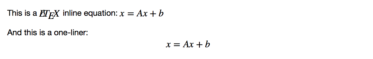
There are several ways to insert LaTeX code in a cell. The easiest way is to simply use the Markdown syntax, wrapping the equations with a single dollar sign, $, for an inline LaTeX formula, or with a double dollar sign, $$, for a one-line central equation. Remember that to have a correct output, the cell should be set as Markdown. Here's an example:
In Markdown:
This is a $LaTeX$ inline equation: $x = Ax+b$

And this is a one-liner: $$x = Ax + b$$
This produces the following output:
If you're looking for something more elaborate, that is, a formula that spans for more than one line, a table, a series of equations that should be aligned, or simply the use of special LaTeX functions, then it's better to use the %%latex magic command offered by the Jupyter Notebook. In this case, the cell must be in code mode and contain the magic command as the first line. The following lines must define a complete LaTeX environment that can be compiled by the LaTeX interpreter.
Here are a couple of examples that show you what you can do:
In:%%latex
   [
    |u(t)| =
     begin{cases}
      u(t) & text{if } t geq 0 \
      -u(t)       & text{otherwise }
     end{cases}
   ]
Here is the output of the first example:

In:%%latex
   begin{align}
   f(x) &= (a+b)^2 \
        &= a^2 + (a+b) + (a+b) + b^2 \
        &= a^2 + 2cdot (a+b) + b^2
   end{align}
The new output when the second example is run is:


Remember that by using the %%latex magic command, the whole cell must comply with the LaTeX syntax. Therefore, if you just need to write a few simple equations in the text, we strongly advise that you use the Markdown method (a text-to-HTML conversion tool for web writers developed by John Gruber, with the help of Aaron Swartz: https://daringfireball.net/projects/markdown/).
Being able to integrate technical formulas in markdown is particularly fruitful for tasks involving the development of code based on data since it automatically accomplishes the often neglected duty of documenting and illustrating how data analysis has been managed as well as its premises, assumptions, and intermediate and final results. If a part of your job is to also present your work and persuade internal or external stakeholders in the project, Jupyter can really do the magic of storytelling for you with little additional effort.
On the web page https://github.com/ipython/ipython/wiki/A-gallery-of-interesting-IPython-Notebooks, there are many examples, some of which you may find inspiring for your work, as it did for ours. Actually, we have to confess that keeping a clean, up-to-date Jupyter Notebook has saved us uncountable times when meeting with managers and stakeholders have suddenly popped up, requiring us to present the state of our work hastily.
In short, Jupyter allows you to do the following:
- See intermediate (debugging) results for each step of the analysis
- Run only some sections (or cells) of the code
- Store intermediate results in JSON format and have the ability to perform version control on them
- Present your work (this will be a combination of text, code, and images), share it via the Jupyter Notebook Viewer service (http://nbviewer.jupyter.org/), and easily export it into HTML, PDF, or even slideshows
In the next section, we will discuss Jupyter's installation in more detail and show an example of its usage in a data science task.
Fast installation and first test usage
Jupyter is our favored choice throughout this book. It is used to clearly and effectively illustrate and narrate operations using scripts and data, and their consequent results.
Though we strongly recommend using Jupyter, if you are using a REPL or an IDE, you can use the same instructions and expect identical results (except for the print formats and extensions of the returned results).
If you do not have Jupyter installed on your system, you can promptly set it up by using the following command:
$> pip install jupyter
You can find complete instructions about Jupyter installation (covering different operating systems) at http://jupyter.readthedocs.io/en/latest/install.html.
After installation, you can immediately start using Jupyter by calling it from the command line:
$> jupyter notebook
Once the Jupyter instance has opened in the browser, click on the New button; in the Notebooks section, choose Python 3 (other kernels may be present in the section depending on what you installed).
At this point, your new empty notebook will look like the following image:
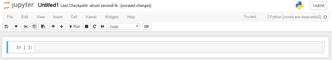
At this point, you can start entering the commands in the first cell. For instance, you may start trying typing the following into the cell where the cursor is flashing:
In: print ("This is a test")
After writing in the cell, you just press the Play button which is below the cell tab (or, as a keyboard hotkey, you can push shift and enter buttons at the same time) to run it and obtain an output. Then, another cell will appear for your input. As you are writing in a cell, if you press the plus button on the menu bar, you will get a new cell, and you can move from one cell to another using the arrows on the menu.
Most of the other functions are quite intuitive, and we invite you to try them. In order to learn how Jupyter works, you may use a quick start guide such as http://jupyter-notebook-beginner-guide.readthedocs.io/en/latest/, or buy a book specializing in Jupyter functionalities.
- IPython Interactive Computing and Visualization Cookbook by Cyrille Rossant, Packt Publishing, September 25, 2014
- Learning IPython for Interactive Computing and Data Visualization by Cyrille Rossant, Packt Publishing, April 25, 2013
For illustrative purposes, just consider that every Jupyter block of instructions has a numbered input statement and an output of one. Therefore, you will find the code presented in this book structured in two blocks, at least when the output is not trivial at all. Otherwise, expect only the input part:
In: <the code you have to enter> Out: <the output you should get>
As a rule, you just have to type the code after In: in your cells and run it. You can then compare your output with the output that we may provide using Out:, followed by the output that we actually obtained on our computers when we tested the code.
Jupyter magic commands
As a special tool for interactive tasks, Jupyter offers special commands that help to better understand the code that you are currently writing.
For instance, some of the commands are as follows:
- * <object>? and <object>??: This prints a detailed description (with ?? being even more verbose) of <object>
- %<function>: This uses the special <magic function>
Let's demonstrate the usage of these commands with an example. We first start the interactive console with the jupyter command, which is used to run Jupyter from the command line, as shown here:
$> jupyter console
   Jupyter Console 4.1.1

In [1]: obj1 = range(10)
Then, in the first line of code, which is marked by Jupyter as [1], we create a list of 10 numbers (from 0 to 9), assigning the output to an object named obj1:
In [2]: obj1?
        Type:        range
        String form: range(0, 10)
        Length:      10
        Docstring:
        range(stop) -> range object
        range(start, stop[, step]) -> range object
        Return an object that produces a sequence of integers from
        start (inclusive)
        to stop (exclusive) by step.  range(i, j) produces i, i+1, i+2,
        ..., j-1.
        start defaults to 0, and stop is omitted!  range(4) produces 0,
        1, 2, 3.
        These are exactly the valid indices for a list of 4 elements.
        When step is given, it specifies the increment (or decrement).

In [3]: %timeit x=100
        The slowest run took 184.61 times longer than the fastest.
        This could mean that an intermediate result is being cached.
        10000000 loops, best of 3: 24.6 ns per loop

In [4]: %quickref
In the next line of code, which is numbered [2], we inspect the obj1 object using the Jupyter command ?. Jupyter introspects the object, prints its details (obj is a range object that can generate the values [1, 2, 3..., 9] and elements), and finally prints some general documentation on the range objects. For complex objects, the usage of ?? instead of ? provides even more verbose output.
In line [3], we use the timeit magic function with a Python assignment (x=100). The timeit function runs this instruction many times and stores the computational time needed to execute it. Finally, it prints the average time that was taken to run the Python function.
We complete the overview with a list of all the possible special Jupyter functions by running the quickref helper function, as shown in line [4].
As you must have noticed, each time we use Jupyter, we have an input cell and, optionally, an output cell if there is something that has to be printed on stdout. Each input is numbered so it can be referenced inside the Jupyter environment itself. For our purposes, we don't need to provide such references in the code of this book. Therefore, we will just report inputs and outputs without their numbers. However, we'll use the generic In: and Out: notations to point out the input and output cells. Just copy the commands after In: to your own Jupyter cell and expect an output that will be reported on the following Out:.
Therefore, the basic notations will be as follows:
- The In: command
- The Out: output (wherever it is present and useful to be reported in this book)
Otherwise, if we expect you to operate directly on the Python console, we will use the following form:
>>> command
Wherever necessary, the command-line input and output will be written as follows:
$> command
Moreover, to run the bash command in the Jupyter console, prefix it with a ! (exclamation mark):
In: !ls
    Applications    Google Drive    Public          Desktop
    Develop
    Pictures        env             temp
    ...

In: !pwd
    /Users/mycomputer
Installing packages directly from Jupyter Notebooks
Jupyter magic commands are really efficient in accomplishing different tasks, but you may sometimes find it difficult to achieve installing new packages during a Jupyter session (and it will happen often since you are using different environments based on conda or env). As Jake VanderPlas explained in his blog post Installing Python Packages from a Jupyter Notebook (https://jakevdp.github.io/blog/2017/12/05/installing-python-packages-from-jupyter/), it is a matter of fact that Jupyter kernels are different from the shell you started from, that is, you may be upgrading a wrong environment when you issue magic commands such as !pip install numpy or !conda install --yes numpy.
The correct approach for installing, let's say, NumPy, using pip under a Jupyter Notebook is by creating a cell like this:
In: import sys
    !"{sys.executable}" -m pip install numpy
Instead, if you want to use conda, this is the cell you have to create:
In: import sys
    !conda install --yes --prefix "{sys.prefix}" numpy
Just replace numpy with any package you would like to install and then run, and the installation is guaranteed to succeed.
Checking the new JupyterLab environment
If you feel like using JupyterLab and want to be a precursor of using the interface that will become a standard in a short time, you can just switch from issuing $> jupyter notebook to $> jupyter lab. JupyterLab will start automatically on your browser at the http://localhost:8888 address:
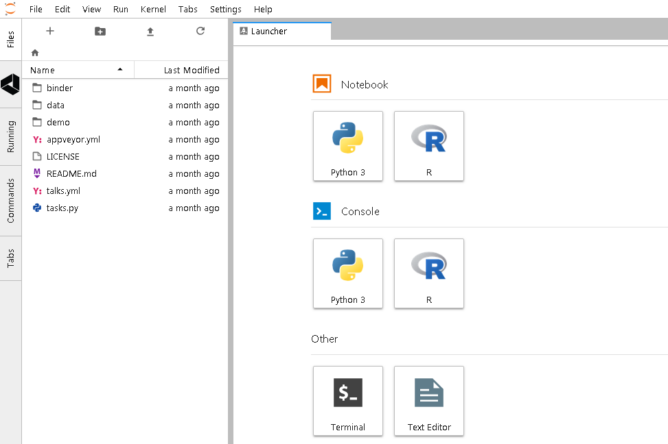
You will be welcomed by a user interface composed of a launcher, where you can find many starting options represented as icons (in the original interface they were menu items), and a series of tabs offering direct access to files on disks, on Google Drive, showing the running kernels and notebooks, and commands for configuring the notebook and formatting the information in it.
Basically, it is an advanced and flexible interface, which is especially useful if you access all such resources on a remote server, allowing you to have everything at a glance on the very same workbench.
How Jupyter Notebooks can help data scientists
The main goal of the Jupyter Notebook is easy storytelling. Storytelling is essential in data science because you must have the power to do the following:
- See intermediate (debugging) results for each step of the algorithm you're developing
- Run only some sections (or cells) of the code
- Store intermediate results and have the ability to version them
- Present your work (this will be a combination of text, code, and images)
Here comes Jupyter; it actually implements all of the preceding actions:
- To launch the Jupyter Notebook, run the following command:
$> jupyter notebook
- A web browser window will pop up on your desktop, backed by a Jupyter server instance. This is what the main window looks like:
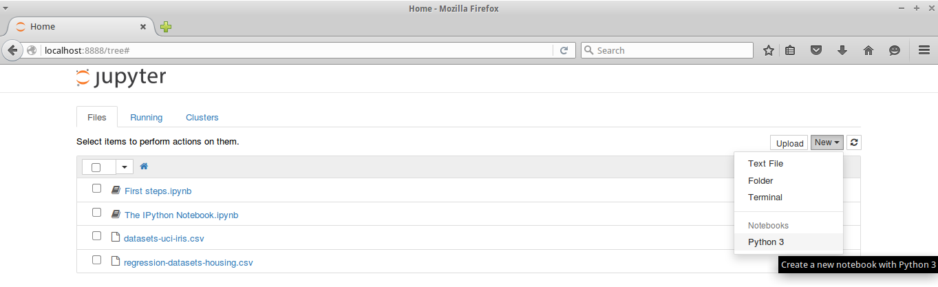
-
Then, click on New Notebook. A new window will open, as shown in the following screenshot. You can start using the notebook as soon as the kernel is ready. The small circle on the top right, below the Python icon, indicates the state of the kernel: if it's filled, it means that the kernel is busy working; if it's empty (like the one in the screenshot), it means that the kernel is in idle, that is, ready to run any code:
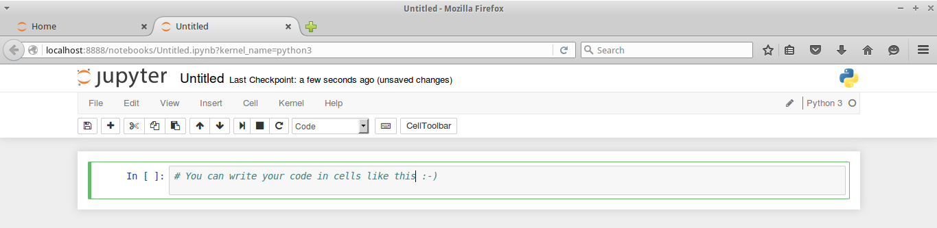
This is the web app that you'll use to compose your story. It's very similar to a Python IDE, with the bottom section (where you can write the code) composed of cells.
A cell can be either a piece of text (eventually formatted with a markup language) or a piece of code. In the second case, you have the ability to run the code, and any eventual output (the standard output) will be placed under the cell. The following is a very simple example of the same:
In: import random
    a = random.randint(0, 100)
    a

Out: 16

In: a*2

Out: 32
In the first cell, which is denoted by In:, we import the random module, assign a random value between 0 and 100 to the variable a, and print the value. When this cell is run, the output, which is denoted as Out:, is the random number. Then, in the next cell, we will just print the double of the value of the variable a.
As you can see, it's a great tool for debugging and deciding which parameter is best for a given operation. Now, what happens if we run the code in the first cell? Will the output of the second cell being modified since a is different? Actually, no, it won't. Each cell is independent and autonomous. In fact, after we run the code in the first cell, we end up with this inconsistent status:
In: import random
    a = random.randint(0, 100)
    a

Out: 56

In: a*2

Out: 32
Jupyter is a simple, flexible, and powerful tool. However, as seen in the preceding example, you must note that when you update a variable that is going to be used later on in your Notebook, remember to run all the cells following the updated code so that you have a consistent state.
When you save a Jupyter Notebook, the resulting .ipynb file is JSON formatted, and it contains all the cells and their content plus the output. This makes things easier because you don't need to run the code to see the notebook (actually, you also don't need to have Python and its set of toolkits installed). This is very handy, especially when you have pictures featured in the output and some very time-consuming routines in the code. A downside of using the Jupyter Notebook is that its file format, which is JSON structured, cannot be easily read by humans. In fact, it contains images, code, text, and so on.
Now, let's discuss a data science-related example (don't worry about understanding it completely):
In: %matplotlib inline
    import matplotlib.pyplot as plt
    from sklearn import datasets
    from sklearn.feature_selection import SelectKBest, f_regression
    from sklearn.linear_model import LinearRegression
    from sklearn.svm import SVR
    from sklearn.ensemble import RandomForestRegressor
In the following cell, some Python modules are imported:
In: boston_dataset = datasets.load_boston()
    X_full = boston_dataset.data
    Y = boston_dataset.target
    print (X_full.shape)
    print (Y.shape)

Out:(506, 13)
    (506,)
Then, in cell [2], the dataset is loaded and an indication of its shape is shown. The dataset contains 506 house values that were sold in the suburbs of Boston, along with their respective data arranged in columns. Each column of the data represents a feature. A feature is a characteristic property of the observation. Machine learning uses features to establish models that can turn them into predictions. If you are from a statistical background, you can add features that can be intended as variables (values that vary with respect to the observations).
To see a complete description of the dataset, use print boston_dataset.DESCR.
After loading the observations and their features, in order to provide a demonstration of how Jupyter can effectively support the development of data science solutions, we will perform some transformations and analysis on the dataset. We will use classes, such as SelectKBest, and methods, such as .getsupport() or .fit(). Don't worry whether these are not clear to you now; they will all be covered extensively later in this book. Try to run the following code:
In: selector = SelectKBest(f_regression, k=1)
    selector.fit(X_full, Y)
    X = X_full[:, selector.get_support()]
    print (X.shape)

Out:(506, 1)
For In:, we select a feature (the most discriminative one) of the SelectKBest class that is fitted to the data by using the .fit() method. Thus, we reduce the dataset to a vector with the help of a selection operated by indexing on all the rows and on the selected feature, which can be retrieved by the .get_support() method.
Since the target value is a vector, we can, therefore, try to see whether there is a linear relationship between the input (the feature) and the output (the house value). When there is a linear relationship between two variables, the output will constantly react to changes in the input by the same proportional amount and direction:
In: def plot_scatter(X,Y,R=None):
        plt.scatter(X, Y, s=32, marker='o', facecolors='white')
        if R is not None:
                plt.scatter(X, R, color='red', linewidth=0.5)
        plt.show()

In: plot_scatter(X,Y)
The following is the output obtained after executing the preceding command:
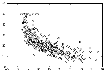
In our example, as X increases, Y decreases. However, this does not happen at a constant rate, because the rate of change is intense up to a certain X value, and then it decreases and becomes constant. This is a condition of nonlinearity, and we can further visualize it using a regression model. This model hypothesizes that the relationship between X and Y is linear in the form of y=a+bX. Its a and b parameters are estimated according to certain criteria.
In the fourth cell, we scatter the input and output values for this problem:
In: regressor = LinearRegression(normalize=True).fit(X, Y)
    plot_scatter(X, Y, regressor.predict(X))
The following is the output obtained after executing the preceding code:
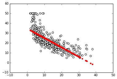
In the next cell, we create a regressor (a simple linear regression with feature normalization), train the regressor, and finally plot the best linear relation (that's the linear model of the regressor) between the input and output. Clearly, the linear model is an approximation that is not working well. We have two possible paths that we can follow at this point. We can transform the variables in order to make their relationship linear, or we can use a nonlinear model. Support Vector Machine (SVM) is a class of models that can easily solve nonlinearities. Also, Random Forests is another model for automatic solving of similar problems. Let's see them in action in Jupyter:
In: regressor = SVR().fit(X, Y)
    plot_scatter(X, Y, regressor.predict(X))
The following is the output obtained after executing the preceding code:
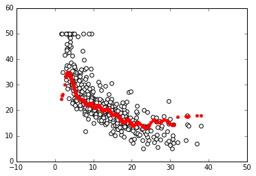
Now we proceed using the even more sophisticated algorithm, the Random Forests regressor:
In: regressor = RandomForestRegressor().fit(X, Y)
    plot_scatter(X, Y, regressor.predict(X))
The following is the output obtained after executing the preceding code:

Finally, in the last two cells, we will repeat the same procedure. This time, we will use two nonlinear approaches: an SVM and a Random Forest-based regressor.
This demonstrative code solves the nonlinearity problem. At this point, it is very easy to change the selected feature, regressor, and the number of features we use to train the model, and so on by simply modifying the cells where the script is. Everything can be done interactively, and according to the results we see, we can decide on both what should be kept or changed and what is to be done next.
Alternatives to Jupyter
If you don't like using Jupyter, there are actually a few alternatives that can help you test the code you will find in this book. If you have experience with R, the RStudio (http://www.rstudio.com/) layout may appeal more to you. In this case, Yhat, a company providing data science solutions for decision APIs, offers their data science IDE for Python free of charge, named Rodeo (http://www.yhat.com/products/rodeo). Rodeo works by using the IPython kernel of Jupyter under the hood, yet it is an interesting alternative given its different user interface.
The main advantages of using Rodeo are as follows:
- A video layout arranged in four Windows: editor, console, plots, and environment
- Autocomplete for the editor and console
- Plots are always visible inside the application in a specific Window
- You can easily inspect the working variables in the environment Window
Rodeo can be simply installed using the installer. You can download it from its website, or you can simply use the following in the command line:
$> pip install rodeo
After the installation, you can immediately run the Rodeo IDE with the following command:
$> rodeo .
Instead, if you have experience with MATLAB from Mathworks, you will find it easier to work with Spyder (http://pythonhosted.org/spyder/), a scientific IDE that can be found in major Scientific Python distributions (it is present in Anaconda, WinPython, and Python (x, y)—all distributions that we have suggested in this book). If you don't use a distribution, in order to install Spyder, you have to follow the instructions that can be found at http://pythonhosted.org/spyder/installation.html. Spyder allows for advanced editing, interactive editing, debugging, and introspection features, and your scripts can be run in a Jupyter console or in a shell-like environment.
Datasets and code used in this book
As we progress through the concepts presented in this book, in order to facilitate the reader's understanding, learning, and memorizing processes, we will illustrate practical and effective data science Python applications on various explicative datasets. The reader will always be able to immediately replicate, modify, and experiment with the proposed instructions and scripts on the data that we will use in this book.
As for the code that you are going to find in this book, we will limit our discussions to the most essential commands in order to inspire you from the beginning of your data science journey with Python to do more with less by leveraging key functions from the packages we presented beforehand.
Given our previous introduction, we will present the code to be run interactively as it appears on a Jupyter console or Notebook.
All the presented code will be offered in Notebooks, which is available on the Packt website (as pointed out in the Preface). As for the data, we will provide different examples of datasets.
Scikit-learn toy datasets
The Scikit-learn toy dataset module is embedded in the Scikit-learn package. Such datasets can easily be directly loaded into Python by the import command, and they don't require any download from any external internet repository. Some examples of this type of dataset are the Iris, Boston, and Digits datasets, to name the principal ones mentioned in uncountable publications and books, and a few other classic ones for classification and regression.
Structured in a dictionary-like object, besides the features and target variables, they offer complete descriptions and contextualization of the data itself.
For instance, to load the Iris dataset, enter the following commands:
In: from sklearn import datasets
    iris = datasets.load_iris()
After loading the dataset, we can explore the data description and understand how the features and targets are stored. All Scikit-learn datasets present the following methods:
- .DESCR: This provides a general description of the dataset
- .data: This contains all the features
- .feature_names: This reports the names of the features
- .target: This contains the target values, expressed as values or numbered classes
- .target_names: This reports the names of the classes in the target
- .shape: This is a method that you can apply to both .data and .target; it reports the number of observations (the first value) and features (the second value, if present) that are present
Now, let's just try to implement them (no output is reported, but the print commands will provide you with plenty of information):
In: print (iris.DESCR)
    print (iris.data)
    print (iris.data.shape)
    print (iris.feature_names)
    print (iris.target)
    print (iris.target.shape)
    print (iris.target_names)
You should know something else about the dataset—how many examples and variables are present, and what their names are. Notice that the main data structures that are enclosed in the iris object are the two arrays, data, and target:
In: print (type(iris.data))

Out: <class 'numpy.ndarray'>
Iris.data offers the numeric values of the variables named sepal length, sepal width, petal length, and petal width, arranged in a matrix form (150,4), where 150 is the number of observations and 4 is the number of features. The order of the variables is the order presented in iris.feature_names.
Iris.target is a vector of integer values, where each number represents a distinct class (refer to the content of target_names; each class name is related to its index number and setosa, which is the zero element of the list, is represented as 0 in the target vector).
The Iris flower dataset was first used in 1936 by Ronald Fisher, who was one of the fathers of modern statistical analysis, in order to demonstrate the functionality of linear discriminant analysis on a small set of empirically verifiable examples (each of the 150 data points represented iris flowers). These examples were arranged into tree-balanced species classes (each class consisted of one-third of the examples) and were provided with four metric descriptive variables that, when combined, were able to separate the classes.
The advantage of using such a dataset is that it is very easy to load, handle, and explore for different purposes, from supervised learning to a graphical representation. Modeling activities take almost no time on any computer, no matter what its specifications are. Moreover, the relationship between the classes and the role of the explicative variables are well-known. Therefore, the task is challenging, but it is not very arduous.
For example, let's just observe how classes can be easily separated when you wish to combine at least two of the four available variables by using a scatterplot matrix.
Scatterplot matrices are arranged in a matrix format, whose columns and rows are the dataset variables. The elements of the matrix contain single scatterplots whose x values are determined by the row variable of the matrix and y values by the column variable. The diagonal elements of the matrix may contain a distribution histogram or some other univariate representation of the variable at the same time in its row and column.
The pandas library offers an off-the-shelf function to quickly build scatterplot matrices and start exploring relationships and distributions between the quantitative variables in a dataset:
In: import pandas as pd
    import numpy as np
    colors = list()
    palette = {0: "red", 1: "green", 2: "blue"}

In: for c in np.nditer(iris.target): colors.append(palette[int(c)])
        # using the palette dictionary, we convert
        # each numeric class into a color string
    dataframe = pd.DataFrame(iris.data,  columns=iris.feature_names)

In: sc = pd.scatter_matrix(dataframe, alpha=0.3, figsize=(10, 10),
    diagonal='hist', color=colors, marker='o', grid=True)
The following is the output obtained after executing the preceding code:
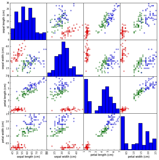
We encourage you to experiment a lot with this dataset and with similar ones before you work on other complex real data because the advantage of focusing on an accessible, non-trivial data problem is that it can help you to quickly build your foundations on data science.
After a while anyway, though they are useful and interesting for your learning activities, toy datasets will start limiting the variety of different experimentations that you can achieve. In spite of the insights provided, in order to progress, you'll need to gain access to complex and realistic data science topics. Consequently, we will have to resort to some external data.
The MLdata.org and other public repositories for open source data
The second type of example dataset that we will present can be downloaded directly from the machine learning dataset repository, or from the LIBSVM data website. Contrary to the previous dataset, in this case, you will need access to the internet.
First, mldata.org is a public repository for machine learning datasets that is hosted by the TU Berlin University and supported by Pattern Analysis, Statistical Modelling, and Computational Learning (PASCAL), a network funded by the European Union. You are free to download any dataset from this repository and experiment with it.
For example, if you need to download all the data related to earthquakes since 1972, as reported by the United States Geological Survey, in order to analyze the data to search for predictive patterns, you will find the data repository at http://mldata.org/repository/data/viewslug/global-earthquakes/ (here, you will find a detailed description of the data).
Note that the directory that contains the dataset is global-earthquakes; you can directly obtain the data by using the following commands:
In: from sklearn.datasets import fetch_mldata
    earthquakes = fetch_mldata('global-earthquakes')
    print (earthquakes.data)
    print (earthquakes.data.shape)

Out: (59209L, 4L)
As in the case of the Scikit-learn package toy dataset, the obtained object is a complex dictionary-like structure, where your predictive variables are earthquakes.data and your target to be predicted is earthquakes.target. This being the real data, in this case, you will have quite a lot of examples and just a few variables available.
LIBSVM data examples
LIBSVM Data (http://www.csie.ntu.edu.tw/~cjlin/libsvmtools/datasets/) is a page that gathers data from many other collections. It is maintained by Chih-Jen Lin, one of the authors of LIBSVM, a support vector machines learning algorithm for predictions (Chih-Chung Chang and Chih-Jen Lin,
LIBSVM : a library for support vector machines. ACM Transactions on Intelligent Systems and Technology, 2:27:1--27:27, 2011
). This offers different regression, binary, and multilabel classification datasets that are stored in the LIBSVM format. This repository is quite interesting if you wish to experiment with the support vector machine's algorithm, and, again, it is free for you to download and use the data.
If you want to load a dataset, first go to the web page where you can visualize the data on your browser. In the case of our example, visit http://www.csie.ntu.edu.tw/~cjlin/libsvmtools/datasets/binary/a1a and note down the address (a1a is a dataset that's originally from the UC Irvine Machine Learning Repository, another open source data repository). Then, you can proceed by performing a direct download using that address:
In: import urllib2
    url =
    'http://www.csie.ntu.edu.tw/~cjlin/libsvmtools/datasets/binary/a1a'
    a2a = urllib2.urlopen(url)

In: from sklearn.datasets import load_svmlight_file
    X_train, y_train = load_svmlight_file(a2a)
    print (X_train.shape, y_train.shape)

Out: (1605, 119) (1605,)
In return, you will get two single objects: a set of training examples in a sparse matrix format and an array of responses.
Loading data directly from CSV or text files
Sometimes, you may have to download the datasets directly from their repository by using a web browser or a wget command (on Linux systems).
If you have already downloaded and unpacked the data (if necessary) into your working directory, the simplest way to load your data and start working is offered by the NumPy and the pandas library with their respective loadtxt and read_csv functions.
For instance, if you intend to analyze the Boston housing data and use the version present at http://mldata.org/repository/data/viewslug/regression-datasets-housing, you first have to download the regression-datasets-housing.csv file in your local directory.
You can use the following link for a direct download of the dataset: http://mldata.org/repository/data/download/csv/regression-datasets-housing.
Since the variables in the dataset are all numeric (13 continuous and one binary), the fastest way to load and start using it is by trying out the loadtxt NumPy function and directly loading all the data into an array.
Even in real-life datasets, you will often find mixed types of variables, which can be addressed by pandas.read_table or pandas.read_csv. Data can then be extracted by the values method; loadtxt can save a lot of memory if your data is already numeric. In fact, the loadtxt command doesn't require any in-memory duplication:
In: housing = np.loadtxt('regression-datasets-housing.csv',
    delimiter=',')
    print (type(housing))

Out: <class 'numpy.ndarray'>

In: print (housing.shape)

Out: (506, 14)
The loadtxt function expects, by default, tabulation as a separator between the values on a file. If the separator is a colon (,) or a semicolon(;), you have to make it explicit by using the parameter delimiter:
>>>  import numpy as np
>>> type(np.loadtxt)
    <type 'function'>
>>> help(np.loadtxt)
Another important default parameter is dtype, which is set to float.
If you need to determinate a different type (for example, int), you have to declare it beforehand.
For instance, if you want to convert numeric data to int, use the following code:
In: housing_int =housing.astype(int)
Printing the first three elements of the row of the housing and housing_int arrays can help you understand the difference:
In:  print (housing[0,:3], 'n', housing_int[0,:3])

Out: [  6.32000000e-03   1.80000000e+01   2.31000000e+00]
     [ 0 18  2]
Frequently, though not always the case in our example, the data on files feature in the first line of a textual header contains the name of the variables. In this situation, the parameter that is skipped will point out the row in the loadtxt file from where it will start reading the data. Being the header on row 0 (in Python, counting always starts from 0), the skip=1 parameter will save the day and allow you to avoid an error and fail to load your data.
The situation would be slightly different if you were to download the Iris dataset, which is present at http://mldata.org/repository/data/viewslug/datasets-uci-iris/. In fact, this dataset presents a qualitative target variable, class, which is a string that expresses the iris species. Specifically, it's a categorical variable with four levels.
Therefore, if you were to use the loadtxt function, you will get a value error because an array must have all its elements of the same type. The variable class is a string, whereas the other variables are constituted by floating-point values.
The pandas library offers the solution to this and many similar cases, thanks to its DataFrame data structure that can easily handle datasets in a matrix form (row per columns) that is made up of different types of variables.
First, just download the datasets-uci-iris.csv file and have it saved in your local directory.
The dataset can be downloaded from http://archive.ics.uci.edu/ml/machine-learning-databases/iris/. This archive is the UC Irvine Machine Learning Repository, which currently maintains 440 datasets as a service to the machine learning community. Apart from this Iris dataset, you are free to download and try any other dataset present in the repository.
At this point, using read_csv from pandas is quite straightforward:
In: iris_filename = 'datasets-uci-iris.csv'
    iris = pd.read_csv(iris_filename, sep=',', decimal='.',
    header=None, names= ['sepal_length', 'sepal_width', \
    'petal_length', 'petal_width', 'target'])
    print (type(iris))

Out: <class 'pandas.core.frame.DataFrame'>
In order to not make the snippets of code printed in this book too cumbersome, we often wrap it and make it nicely formatted. When necessary, in order to safely interrupt the code and wrap it to a new line, we use the backslash symbol \ as in the preceding code example. When rendering the code of the book by yourself, you can ignore backslash symbols and go on writing all of the instructions on the same line, or you can digit the backslash and start a new line continuing with the code instructions. Please be warned that typing the backslash and then continuing the instruction on the same line will cause an execution error.
Apart from the filename, you can specify the separator (sep), the way the decimal points are expressed (decimal), whether there is a header (in this case, header=None; normally, if you have a header, then header=0), and the name of the variable where there is one (you can use a list; otherwise, pandas will provide some automatic naming).
At this point, if you need to convert the pandas DataFrame into a couple of NumPy arrays that contain the data and target values, this can be done easily in a couple of commands:
In: iris_data = iris.values[:,:4]
    iris_target, iris_target_labels = pd.factorize(iris.target)
    print (iris_data.shape, iris_target.shape)

Out: (150, 4) (150,)
Scikit-learn sample generators
As a last learning resource, the Scikit-learn package also offers the possibility to quickly create synthetic datasets for regression, binary and multilabel classification, cluster analysis, and dimensionality reduction.
The main advantage of recurring synthetic data lies in its instantaneous creation in the working memory of your Python console. It is, therefore, possible to create bigger data examples without having to engage in long downloading sessions from the internet (and saving a lot of stuff on your disk).
For example, you may need to work on a classification problem involving a million data points:
In: from sklearn import datasets
    X,y = datasets.make_classification(n_samples=10**6,
    n_features=10, random_state=101)
    print (X.shape,  y.shape)

Out: (1000000, 10) (1000000,)
After importing just the datasets module, we ask, using the make_classification command, for one million examples (the n_samples parameter) and 10 useful features (n_features). The random_state should be 101, so we are assured that we can replicate the same datasets at a different time and in a different machine.
For instance, you can type the following command:
In: datasets.make_classification(1, n_features=4, random_state=101)
This will always give you the following output:
Out: (array([[-3.31994186, -2.39469384, -2.35882002,  1.40145585]]),
      array([0]))
No matter what the computer and the specific situation are, random_state assures deterministic results that make your experimentations perfectly replicable.
Defining the random_state parameter using a specific integer number (in this case, it's 101, but it may be any number that you prefer or find useful) allows easy replication of the same dataset on your machine, the way it is set up, on different operating systems, and on different machines.
By the way, did it take too long?
On a i3-2330M CPU @ 2.20 GHz machine, it takes this:
In: %timeit X,y = datasets.make_classification(n_samples=10**6,
    n_features=10, random_state=101)

Out: 1 loops, best of 3: 1.17 s per loop
If it doesn't seem like it did take too long on your machine, and if you are ready, having set up and tested everything up to this point, we can start our data science journey.
Summary
In this introductory chapter, we installed everything that we will be using throughout this book, from Python packages to examples. They were installed either directly or by using a scientific distribution. We also introduced Jupyter Notebooks and demonstrated how you can have access to the data run in the tutorials.
In the next chapter, Data Munging, we will have an overview of the data science pipeline and explore all the key tools to handle and prepare data before you apply any learning algorithm and set up your hypothesis experimentation schedule.