


 Download code from GitHub
This chapter gives you an overview of the tools available for data analysis in Python, with details concerning the Python packages and libraries that will be used in this book. A few installation tips are given, and the chapter concludes with a brief example. We will concentrate on how to read data files, select data, and produce simple plots, instead of delving into numerical data analysis.
We assume that you have familiarity with Python and have already developed and run some scripts or used Python interactively, either in the shell or on another interface, such as the Jupyter Notebook (formerly known as the IPython notebook). Hence, we also assume that you have a working installation of Python. In this book, we assume that you have installed Python 3.4 or later.
We also assume that you have developed your own workflow with Python, based on needs and available environment. To follow the examples in this book, you are expected to have access to a working installation of Python 3.4 or later. There are two alternatives to get started, as outlined in the following list:
Use a Python installation from scratch. This can be downloaded from https://www.python.org . This will require a separate installation for each of the required libraries.
Install a prepackaged distribution containing libraries for scientific and data computing. Two popular distributions are Anaconda Scientific Python ( https://store.continuum.io/cshop/anaconda ) and Enthought distribution ( https://www.enthought.com ).
Tip
Even if you have a working Python installation, you might want to try one of the prepackaged distributions. They contain a well-rounded collection of packages and modules suitable for data analysis and scientific computing. If you choose this path, all the libraries in the next list are included by default.
We also assume that you have the libraries in the following list:
numpyandscipy: These are available at http://www.scipy.org . These are the essential Python libraries for computational work. NumPy defines a fast and flexible array data structure, and SciPy has a large collection of functions for numerical computing. They are required by some of the libraries mentioned in the list.matplotlib: This is available at http://matplotlib.org . It is a library for interactive graphics built on top of NumPy. I recommend versions above 1.5, which is what is included in Anaconda Python by default.pandas: This is available at http://pandas.pydata.org . It is a Python data analysis library. It will be used extensively throughout the book.pymc: This is a library to make Bayesian models and fitting in Python accessible and straightforward. It is available at http://pymc-devs.github.io/pymc/ . This package will mainly be used in Chapter 6 , Bayesian Methods, of this book.scikit-learn: This is available at http://scikit-learn.org. It is a library for machine learning in Python. This package is used in Chapter 7, Supervised and Unsupervised Learning.IPython: This is available at http://ipython.org. It is a library providing enhanced tools for interactive computations in Python from the command line.Jupyter: This is available at https://jupyter.org/ . It is the notebook interface working on top of IPython (and other programming languages). Originally part of the IPython project, the notebook interface is a web-based platform for computational and data science that allows easy integration of the tools that are used in this book.
Notice that each of the libraries in the preceding list may have several dependencies, which must also be separately installed. To test the availability of any of the packages, start a Python shell and run the corresponding import statement. For example, to test the availability of NumPy, run the following command:
import numpy
If NumPy is not installed in your system, this will produce an error message. An alternative approach that does not require starting a Python shell is to run the command line:
python -c 'import numpy'
We also assume that you have either a programmer's editor or Python IDE. There are several options, but at the basic level, any editor capable of working with unformatted text files will do.
Most examples in this book will use the Jupyter Notebook interface. This is a browser-based interface that integrates computations, graphics, and other forms of media. Notebooks can be easily shared and published, for example, http://nbviewer.ipython.org/ provides a simple publication path.
It is not, however, absolutely necessary to use the Jupyter interface to run the examples in this book. We strongly encourage, however, that you at least experiment with the notebook and its many features. The Jupyter Notebook interface makes it possible to mix formatted, descriptive text with code cells that evaluate at the same time. This feature makes it suitable for educational purposes, but it is also useful for personal use as it makes it easier to add comments and share partial progress before writing a full report. We will sometimes refer to a Jupyter Notebook as just a notebook.
To start the notebook interface, run the following command line from the shell or Anaconda command prompt:
jupyter notebook
The notebook server will be started in the directory where the command is issued. After a while, the notebook interface will appear in your default browser. Make sure that you are using a standards-compliant browser, such as Chrome, Firefox, Opera, or Safari. Once the Jupyter dashboard shows on the browser, click on the New button on the upper-right side of the page and select Python 3. After a few seconds, a new notebook will open in the browser. A useful place to learn about the notebook interface is http://jupyter.org.
There are some modules that we will need to load at the start of every project. Assuming that you are running a Jupyter Notebook, the required imports are as follows:
%matplotlib inline
import matplotlib.pyplot as plt
import numpy as np
import pandas as pd
Enter all the preceding commands in a single notebook cell and press Shift + Enter to run the whole cell. A new cell will be created when there is none after the one you are running; however, if you want to create one yourself, the menu or keyboard shortcut Ctrl +M+A/B is handy (A for above, B for below the current cell). In Appendix, More on Jupyter Notebook and matplotlib Styles, we cover some of the keyboard shortcuts available and installable extensions (that is, plugins) for Jupyter Notebook.
The statement %matplotlib inline is an example of Jupyter Notebook magic and sets up the interface to display plots inline, that is, embedded in the notebook. This line is not needed (and causes an error) in scripts. Next, optionally, enter the following commands:
import os
plt.style.use(os.path.join(os.getcwd(), 'mystyle.mplstyle') )
As before, run the cell by pressing Shift +Enter. This code has the effect of selecting matplotlib stylesheet mystyle.mplstyle. This is a custom style sheet that I created, which resides in the same folder as the notebook. It is a rather simple example of what can be done; you can modify it to your liking. As we gain experience in drawing figures throughout the book, I encourage you to play around with the settings in the file. There are also built-in styles that you can by typing plt.style.available in a new cell.
This is it! We are all set to start the fun part!
The purpose of this example is to check whether everything is working in your installation and give a flavor of what is to come. We concentrate on the Pandas library, which is the main tool used in Python data analysis.
We will use the MovieTweetings 50K movie ratings dataset, which can be downloaded from https://github.com/sidooms/MovieTweetings. The data is from the study MovieTweetings: a Movie Rating Dataset Collected From Twitter - by Dooms, De Pessemier and Martens presented during Workshop on Crowdsourcing and Human Computation for Recommender Systems, CrowdRec at RecSys (2013). The dataset is spread in several text files, but we will only use the following two files:
ratings.dat: This is a double colon-separated file containing the ratings for each user and moviemovies.dat: This file contains information about the movies
To see the contents of these files, you can open them with a standard text editor. The data is organized in columns, with one data item per line. The meanings of the columns are described in the README.md file, distributed with the dataset. The data has a peculiar aspect: some of the columns use a double colon (::) character as a separator, while others use a vertical bar (|). This emphasizes a common occurrence with real-world data: we have no control on how the data is collected and formatted. For data stored in text files, such as this one, it is always a good strategy to open the file in a text editor or spreadsheet software to take a look at the data and identify inconsistencies and irregularities.
To read the ratings file, run the following command:
    cols = ['user id', 'item id', 'rating', 'timestamp']
ratings = pd.read_csv('data/ratings.dat', sep='::',
                          index_col=False, names=cols,
                          encoding="UTF-8")
The first line of code creates a Python list with the column names in the dataset. The next command reads the file, using the read_csv() function, which is part of Pandas. This is a generic function to read column-oriented data from text files. The arguments used in the call are as follows:
data/ratings.dat: This is the path to file containing the data (this argument is required).sep='::': This is the separator, a double colon character in this case.index_col=False: We don't want any column to be used as an index. This will cause the data to be indexed by successive integers, starting with 1.names=cols: These are the names to be associated with the columns.
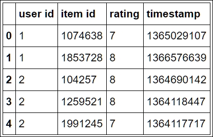
The read_csv() function returns a DataFrame object, which is the Pandas data structure that represents tabular data. We can view the first rows of the data with the following command:
ratings[:5]
This will output a table, as shown in the following image:
To start working with the data, let us find out how many times each rating appears in the table. This can be done with the following commands:
rating_counts = ratings['rating'].value_counts()
rating_counts
The first line of code computes the counts and stores them in the rating_counts variable. To obtain the count, we first use the ratings['rating'] expression to select the rating column from the table ratings. Then, the value_counts() method is called to compute the counts. Notice that we retype the variable name, rating_counts, at the end of the cell. This is a common notebook (and Python) idiom to print the value of a variable in the output area that follows each cell. In a script, it has no effect; we could have printed it with the print command,(print(rating_counts)), as well. The output is displayed in the following image:
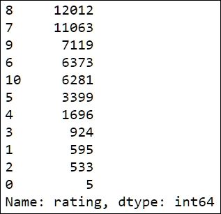
Notice that the output is sorted according to the count values in descending order. The object returned by value_counts is of the Series type, which is the Pandas data structure used to represent one-dimensional, indexed, data. The Series objects are used extensively in Pandas. For example, the columns of a DataFrame object can be thought as Series objects that share a common index.
In our case, it makes more sense to sort the rows according to the ratings. This can be achieved with the following commands:
sorted_counts = rating_counts.sort_index()
sorted_counts
This works by calling the sort_index() method of the Series object, rating_counts. The result is stored in the sorted_counts variable. We can now get a quick visualization of the ratings distribution using the following commands:
sorted_counts.plot(kind='bar', color='SteelBlue')
plt.title('Movie ratings')
plt.xlabel('Rating')
plt.ylabel('Count')
The first line produces the plot by calling the plot() method for the sorted_counts object. We specify the kind='bar' option to produce a bar chart. Notice that we added the color='SteelBlue' option to select the color of the bars in the histogram. SteelBlue is one of the HTML5 color names (for example,
http://matplotlib.org/examples/color/named_colors.html
) available in matplotlib. The next three statements set the title, horizontal axis label, and vertical axis label respectively. This will produce the following plot:
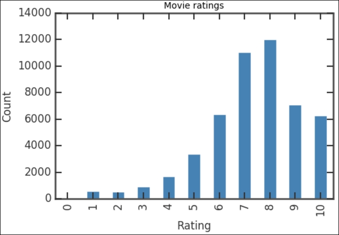
The vertical bars show how many voters that have given a certain rating, covering all the movies in the database. The distribution of the ratings is not very surprising: the counts increase up to a rating of 8, and the count of 9-10 ratings is smaller as most people are reluctant to give the highest rating. If you check the values of the bar for each rating, you can see that it corresponds to what we had previously when printing the rating_counts object. To see what happens if you do not sort the ratings first, plot the rating_counts object, that is, run rating_counts.plot(kind='bar', color='SteelBlue') in a cell.
Let's say that we would like to know if the ratings distribution for a particular movie genre, say Crime Drama, is similar to the overall distribution. We need to cross-reference the ratings information with the movie information, contained in the movies.dat file. To read this file and store it in a Pandas DataFrame object, use the following command:
    cols = ['movie id','movie title','genre']
    movies = pd.read_csv('data/movies.dat', sep='::',
                         index_col=False, names=cols,
                         encoding="UTF-8")
Tip
Downloading the example code
Detailed steps to download the code bundle are mentioned in the Preface of this book. Please have a look. The code bundle for the book is also hosted on GitHub at https://github.com/PacktPublishing/Mastering-Python-Data-Analysis. We also have other code bundles from our rich catalog of books and videos available at https://github.com/PacktPublishing/. Check them out!
We are again using the read_csv() function to read the data. The column names were obtained from the README.md file distributed with the data. Notice that the separator used in this file is also a double colon, ::. The first few lines of the table can be displayed with the command:
movies[:5]
Notice how the genres are indicated, clumped together with a vertical bar, |, as separator. This is due to the fact that a movie can belong to more than one genre. We can now select only the movies that are crime dramas using the following lines:
drama = movies[movies['genre']=='Crime|Drama']
Notice that this uses the standard indexing notation with square brackets, movies[...]. Instead of specifying a numeric or string index, however, we are using the Boolean movies['genre']=='Crime|Drama' expression as an index. To understand how this works, run the following code in a cell:
is_drama = movies['genre']=='Crime|Drama'
is_drama[:5]
This displays the following output:
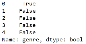
The movies['genre']=='Crime|Drama' expression returns a Series object, where each entry is either True or False, indicating whether the corresponding movie is a crime drama or not, respectively.
Thus, the net effect of the drama = movies[movies['genre']=='Crime|Drama'] assignment is to select all the rows in the movies table for which the entry in the genre column is equal to Crime|Drama and store the result in the drama variable, which is an object of the DataFrame type.
All that we need is the movie id column of this table, which can be selected with the following statement:
drama_ids = drama['movie id']
This, again, uses standard indexing with a string to select a column from a table.
The next step is to extract those entries that correspond to dramas from the ratings table. This requires yet another indexing trick. The code is contained in the following lines:
criterion = ratings['item id'].map(lambda x:(drama_ids==x).any())
drama_ratings = ratings[criterion]
The key to how this code works is the definition of the variable criterion. We want to look up each row of the ratings table and check whether the item id entry is in the drama_ids table. This can be conveniently done by the map() method. This method applies a function to all the entries of a Series object. In our example, the function is as follows:
lambda x:(drama_ids==x).any()
This function simply checks whether an item appears in drama_ids, and if it does, it returns True. The resulting object criterion will be a Series that contains the True value only in the rows that correspond to dramas. You can view the first rows with the following code:
criterion[:10]
We then use the criterion object as an index to select the rows from the ratings table.
We are now done with selecting the data that we need. To produce a rate count and bar chart, we use the same commands as before. The details are in the following code, which can be run in a single execution cell:
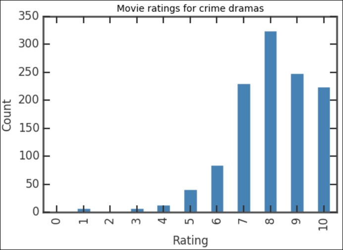
rating_counts = drama_ratings['rating'].value_counts()
sorted_counts = rating_counts.sort_index()
sorted_counts.plot(kind='bar', color='SteelBlue')
plt.title('Movie ratings for dramas')
plt.xlabel('Rating')
plt.ylabel('Count')
As before, this code first computes the counts, indexes them according to the ratings, and then produces a bar chart. This produces a graph that seems to be similar to the overall ratings distribution, as shown in the following figure:
In this chapter, we have seen what tools are available for data analysis in Python, reviewed issues related to installation and workflow, and considered a simple example that requires reading and manipulating data files.
In the next chapter, we will cover techniques to explore data graphically and numerically using some of the main tools provided by the Pandas module.

