


 Download code from GitHub
This chapter kicks off a machine learning (ML) initiative in Scala and Spark. Speaking of Spark, its Machine Learning Library (MLlib) living under the spark.ml package and accessible via its MLlib DataFrame-based API will help us develop scalable data analysis applications. The MLlib DataFrame-based API, also known as Spark ML, provides powerful learning algorithms and pipeline building tools for data analysis. Needless to say, we will, starting this chapter, leverage MLlib's classification algorithms.
The Spark ecosystem, also boasting of APIs to R, Python, and Java in addition to Scala, empowers our readers, be they beginner, or seasoned data professionals, to make sense of and extract analytics from various datasets.
Speaking of datasets, the Iris dataset is the simplest, yet the most famous data analysis task in the ML space. This chapter builds a solution to the data analysis classification task that the Iris dataset represents.
Here is the dataset we will refer to:
- UCI Machine Learning Repository: Iris Data Set
- Accessed July 13, 2018
- Website URL: https://archive.ics.uci.edu/ml/datasets/Iris
The overarching learning objective of this chapter is to implement a Scala solution to the so-called multivariate classification task represented by the Iris dataset.
The following list is a section-wise breakdown of individual learning outcomes:
- A multivariate classification problem
- Project overview—problem formulation
- Getting started with Spark
- Implementing a multiclass classification pipeline
The following section offers the reader an in-depth perspective on the Iris dataset classification problem.
The most famous dataset in data science history is Sir Ronald Aylmer Fisher's classical Iris flower dataset, also known as Anderson's dataset. It was introduced in 1936, as a study in understanding multivariate (or multiclass) classification. What then is multivariate?
The term multivariate can bear two meanings:
- In terms of an adjective, multivariate means having or involving one or more variables.
- In terms of a noun, multivariate may represent a mathematical vector whose individual elements are variate. Each individual element in this vector is a measurable quantity or variable.
Both meanings mentioned have a common denominator variable. Conducting a multivariate analysis of an experimental unit involves at least one measurable quantity or variable. A classic example of such an analysis is the Iris dataset, having one or more (outcome) variables per observation.
In this subsection, we understood multivariate in terms of variables. In the next subsection, we briefly touch upon different kinds of variables, one of them being categorical variables.
In general, variables are of two types:
- Quantitative variable: It is a variable representing a measurement that is quantified by a numeric value. Some examples of quantitative variables are:
- A variable representing the age of a girl called
Huan(Age_Huan). In September of 2017, the variable representing her age contained the value24. Next year, one year later, that variable would be the number 1 (arithmetically) added to her current age. - The variable representing the number of planets in the solar system (
Planet_Number). Currently, pending the discovery of any new planets in the future, this variable contains the number12. If scientists found a new celestial body tomorrow that they think qualifies to be a planet, thePlanet_Numbervariable's new value would be bumped up from its current value of12to13. - Categorical variable: A variable that cannot be assigned a numerical measure in the natural order of things. For example, the status of an individual in the United States. It could be one of the following values: a citizen, permanent resident, or a non-resident.
In the next subsection, we will describe categorical variables in some detail.
We will draw upon the definition of a categorical variable from the previous subsection. Categorical variables distinguish themselves from quantitative variables in a fundamental way. As opposed to a quantitative variable that represents a measure of a something in numerical terms, a categorical variable represents a grouping name or a category name, which can take one of the finite numbers of possible categories. For example, the species of an Iris flower is a categorical variable and the value it takes could be one value from a finite set of categorical values: Iris-setosa, Iris-virginica, and Iris-versicolor.
It may be useful to draw on other examples of categorical variables; these are listed here as follows:
- The blood group of an individual as in A+, A-, B+, B-, AB+, AB-, O+, or O-
- The county that an individual is a resident of given a finite list of counties in the state of Missouri
- The political affiliation of a United States citizen could take up categorical values in the form of Democrat, Republican, or Green Party
- In global warming studies, the type of a forest is a categorical variable that could take one of three values in the form of tropical, temperate, or taiga
The first item in the preceding list, the blood group of a person, is a categorical variable whose corresponding data (values) are categorized (classified) into eight groups (A, B, AB, or O with their positives or negatives). In a similar vein, the species of an Iris flower is a categorical variable whose data (values) are categorized (classified) into three species groups—Iris-setosa, Iris-versicolor, and Iris-virginica.
That said, a common data analysis task in ML is to index, or encode, current string representations of categorical values into a numeric form; doubles for example. Such indexing is a prelude to a prediction on the target or label, which we shall talk more about shortly.
In respect to the Iris flower dataset, its species variable data is subject to a classification (or categorization) task with the express purpose of being able to make a prediction on the species of an Iris flower. At this point, we want to examine the Iris dataset, its rows, row characteristics, and much more, which is the focus of the upcoming topic.
The Iris flower dataset comprises of a total of 150 rows, where each row represents one flower. Each row is also known as an observation. This 150 observation Iris dataset is made up of three kinds of observations related to three different Iris flower species. The following table is an illustration:

Iris dataset observation breakup table
Referring to the preceding table, it is clear that three flower species are represented in the Iris dataset. Each flower species in this dataset contributes equally to 50 observations apiece. Each observation holds four measurements. One measurement corresponds to one flower feature, where each flower feature corresponds to one of the following:
- Sepal Length
- Sepal Width
- Petal Length
- Petal Width
The features listed earlier are illustrated in the following table for clarity:

Iris features
Okay, so three flower species are represented in the Iris dataset. Speaking of species, we will henceforth replace the term species with the term classes whenever there is the need to stick to an ML terminology context. That means #1-Iris-setosa from earlier refers to Class # 1, #2-Iris-virginica to Class # 2, and #3-Iris-versicolor to Class # 3.
We just listed three different Iris flower species that are represented in the Iris dataset. What do they look like? What do their features look like? These questions are answered in the following screenshot:

Representations of three species of Iris flower
That said, let's look at the Sepal and Petal portions of each class of Iris flower. The Sepal (the larger lower part) and Petal (the lower smaller part) dimensions are how each class of Iris flower bears a relationship to the other two classes of Iris flowers. In the next section, we will summarize our discussion and expand the scope of the discussion of the Iris dataset to a multiclass, multidimensional classification task.
In this section, we will restate the facts about the Iris dataset and describe it in the context of an ML classification task:
- The Iris dataset classification task is multiclass because a prediction of the class of a new incoming Iris flower from the wild can belong to any of three classes.
- Indeed, this chapter is all about attempting a species classification (inferring the target class of a new Iris flower) using sepal and petal dimensions as feature parameters.
- The Iris dataset classification is multidimensional because there are four features.
- There are 150 observations, where each observation is comprised of measurements on four features. These measurements are also known by the following terms:
- Input attributes or instances
- Predictor variables (
X) - Input variables (
X)
- Classification of an Iris flower picked in the wild is carried out by a model (the computed mapping function) that is given four flower feature measurements.
- The outcome of the Iris flower classification task is the identification of a (computed) predicted value for the response from the predictors by a process of learning (or fitting) a discrete number of targets or category labels (
Y). The outcome or predicted value may mean the same as the following: - Categorical response variable: In a later section, we shall see that an indexer algorithm will transform all categorical values to numbers
- Response or outcome variable (
Y)
So far, we have claimed that the outcome (Y) of our multiclass classification task is dependent on inputs (X). Where will these inputs come from? This is answered in the next section.
An integral aspect of our data analysis or classification task we did not hitherto mention is the training dataset. A training dataset is our classification task's source of input data (X). We take advantage of this dataset to obtain a prediction on each target class, simply by deriving optimal perimeters or boundary conditions. We just redefined our classification process by adding in the extra detail of the training dataset. For a classification task, then we have X on one side and Y on the other, with an inferred mapping function in the middle. That brings us to the mapping or predictor function, which is the focus of the next section.
We have so far talked about an input variable (X) and an output variable (Y). The goal of any classification task, therefore, is to discover patterns and find a mapping (predictor) function that will take feature measurements (X) and map input over to the output (Y). That function is mathematically formulated as:
Y = f(x)
This mapping is how supervised learning works. A supervised learning algorithm is said to learn or discover this function. This will be the goal of the next section.
This section starts with a schematic depicting the components of the mapping function and an algorithm that learns the mapping function. The algorithm is learning the mapping function, as shown in the following diagram:

An input to output mapping function and an algorithm learning the mapping function
The goal of our classification process is to let the algorithm derive the best possible approximation of a mapping function by a learning (or fitting) process. When we find an Iris flower out in the wild and want to classify it, we use its input measurements as new input data that our algorithm's mapping function will accept in order to give us a predictor value (Y). In other words, given feature measurements of an Iris flower (the new data), the mapping function produced by a supervised learning algorithm (this will be a random forest) will classify the flower.
Two kinds of ML problems exist that supervised learning classification algorithms can solve. These are as follows:
- Classification tasks
- Regression tasks
In the following paragraph, we will talk about a mapping function with an example. We explain the role played by a "supervised learning classification task" in deducing the mapping function. The concept of a model is introduced.
Let's say we already knew that the (mapping) function f(x) for the Iris dataset classification task is exactly of the form x + 1, then there is there no need for us to find a new mapping function. If we recall, a mapping function is one that maps the relationship between flower features, such as sepal length and sepal width, on the species the flower belongs to? No.
Therefore, there is no preexisting function x + 1 that clearly maps the relationship between flower features and the flower's species. What we need is a model that will model the aforementioned relationship as closely as possible. Data and its classification seldom tend to be straightforward. A supervised learning classification task starts life with no knowledge of what function f(x) is. A supervised learning classification process applies ML techniques and strategies in an iterative process of deduction to ultimately learn what f(x) is.
In our case, such an ML endeavor is a classification task, a task where the function or mapping function is referred to in statistical or ML terminology as a model.
In the next section, we will describe what supervised learning is and how it relates to the Iris dataset classification. Indeed, this apparently simplest of ML techniques finds wide applications in data analysis, especially in the business domain.
At the outset, the following is a list of salient aspects of supervised learning:
- The term supervised in supervised learning stems from the fact that the algorithm is learning or inferring what the mapping function is.
- A data analysis task, either classification or regression.
- It contains a process of learning or inferring a mapping function from a labeled training dataset.
- Our Iris training dataset has training examples or samples, where each example may be represented by an input feature vector consisting of four measurements.
- A supervised learning algorithm learns or infers or derives the best possible approximation of a mapping function by carrying out a data analysis on the training data. The mapping function is also known as a model in statistical or ML terminology.
- The algorithm provides our model with parameters that it learns from the training example set or training dataset in an iterative process, as follows:
- Each iteration produces predicted class labels for new input instances from the wild
- Each iteration of the learning process produces progressively better generalizations of what the output class label should be, and as in anything that has an end, the learning process for the algorithm also ends with a high degree of reasonable correctness on the prediction
- An ML classification process employing supervised learning has algorithm samples with correctly predetermined labels.
- The Iris dataset is a typical example of a supervised learning classification process. The term supervised arises from the fact that the algorithm at each step of an iterative learning process applies an appropriate correction on its previously generated model building process to generate its next best model.
In the next section, we will define a training dataset. In the next section, and in the remaining sections, we will use the Random Forest classification algorithm to run data analysis transformation tasks. One such task worth noting here is a process of transformation of string labels to an indexed label column represented by doubles.
In a preceding section, we noted the crucial role played by the input or training dataset. In this section, we reiterate the importance of this dataset. That said, the training dataset from an ML algorithm standpoint is one that the Random Forest algorithm takes advantage of to train or fit the model by generating the parameters it needs. These are parameters the model needs to come up with the next best-predicted value. In this chapter, we will put the Random Forest algorithm to work on training (and testing) Iris datasets. Indeed, the next paragraph starts with a discussion on Random Forest algorithms or simply Random Forests.
A Random Forest algorithm encompasses decision tree-based supervised learning methods. It can be viewed as a composite whole comprising a large number of decision trees. In ML terminology, a Random Forest is an ensemble resulting from a profusion of decision trees.
A decision tree, as the name implies, is a progressive decision-making process, made up of a root node followed by successive subtrees. The decision tree algorithm snakes its way up the tree, stopping at every node, starting with the root node, to pose a do-you-belong-to-a-certain-category question. Depending on whether the answer is a yes or a no, a decision is made to travel up a certain branch until the next node is encountered, where the algorithm repeats its interrogation. Of course, at each node, the answer received by the algorithm determines the next branch to be on. The final outcome is a predicted outcome on a leaf that terminates.
Speaking of trees, branches, and nodes, the dataset can be viewed as a tree made up of multiple subtrees. Each decision at a node of the dataset and the decision tree algorithm's choice of a certain branch is the result of an optimal composite of feature variables. Using a Random Forest algorithm, multiple decision trees are created. Each decision tree in this ensemble is the outcome of a randomized ordering of variables. That brings us to what random forests are—an ensemble of a multitude of decision trees.
It is to be noted that one decision tree by itself cannot work well for a smaller sample like the Iris dataset. This is where the Random Forest algorithm steps in. It brings together or aggregates all of the predictions from its forest of decision trees. All of the aggregated results from individual decision trees in this forest would form one ensemble, better known as a Random Forest.
We chose the Random Forest method to make our predictions for a good reason. The net prediction formed out of an ensemble of predictions is significantly more accurate.
In the next section, we will formulate our classification problem, and in the Getting started with Spark section that follows, implementation details for the project are given.
The intent of this project is to develop an ML workflow or more accurately a pipeline. The goal is to solve the classification problem on the most famous dataset in data science history.
If we saw a flower out in the wild that we know belongs to one of three Iris species, we have a classification problem on our hands. If we made measurements (X) on the unknown flower, the task is to learn to recognize the species to which the flower (and its plant) belongs.
Categorical variables represent types of data which may be divided into groups. Examples of categorical variables are race, sex, age group, and educational level. While the latter two variables may also be considered in a numerical manner by using exact values for age and highest grade completed, it is often more informative to categorize such variables into a relatively small number of groups.
Analysis of categorical data generally involves the use of data tables. A two-way table presents categorical data by counting the number of observations that fall into each group for two variables, one divided into rows and the other divided into columns.
In a nutshell, the high-level formulation of the classification problem is given as follows:

High-level formulation of the Iris supervised learning classification problem
Note
In the Iris dataset, each row contains categorical data (values) in the fifth column. Each such value is associated with a label (Y).
The formulation consists of the following:
- Observed features
- Category labels
Observed features are also known as predictor variables. Such variables have predetermined measured values. These are the inputs X. On the other hand, category labels denote possible output values that predicted variables can take.
The predictor variables are as follows:
sepal_length: It represents sepal length, in centimeters, used as inputsepal_width: It represents sepal width, in centimeters, used as inputpetal_length: It represents petal length, in centimeters, used as input
petal_width: It represents petal width, in centimeters, used as inputsetosa: It represents Iris-setosa, true or false, used as targetversicolour: It represents Iris-versicolour, true or false, used as targetvirginica: It represents Iris-virginica, true or false, used as target
Four outcome variables were measured from each sample; the length and the width of the sepals and petals.
The total build time of the project should be no more than a day in order to get everything working. For those new to the data science area, understanding the background theory, setting up the software, and getting to build the pipeline could take an extra day or two.
The instructions are for Windows users. Note that to run Spark Version 2 and above, Java Version 8 and above, Scala Version 2.11, Simple Build Tool (SBT) version that is at least 0.13.8 is a prerequisite. The code for the Iris project depends on Spark 2.3.1, the latest distribution at the time of writing this chapter. This version was released on December 1, 2017. Implementations in subsequent chapters would likely be based on Spark 2.3.0, released February 28, 2017. Spark 2.3.0 is a major update version that comes with fixes to over 1,400 tickets.
The Spark 2.0 brought with it a raft of improvements. The introduction of the dataframe as the fundamental abstraction of data is one such improvement. Readers will find that the dataframe abstraction and its supporting APIs enhance their data science and analysis tasks, not to mention this powerful feature's improved performance over Resilient Distributed Datasets (RDDs). Support for RDDs is very much available in the latest Spark release as well.
A note on hardware before jumping to prerequisites. The hardware infrastructure I use throughout in this chapter comprises of a 64-bit Windows Dell 8700 machine running Windows 10 with Intel(R) Core(TM) i7-4770 CPU @ 3.40 GHz and an installed memory of 32 GB.
In this subsection, we document three software prerequisites that must be in place before installing Spark.
Note
At the time of this writing, my prerequisite software setup consisted of JDK 8, Scala 2.11.12, and SBT 0.13.8, respectively. The following list is a minimal, recommended setup (note that you are free to try a higher JDK 8 version and Scala 2.12.x).
Here is the required prerequisite list for this chapter:
- Java SE Development Kit 8
- Scala 2.11.12
- SBT 0.13.8 or above
If you are like me, dedicating an entire box with the sole ambition of evolving your own Spark big data ecosystem is not a bad idea. With that in mind, start with an appropriate machine (with ample space and at least 8 GB of memory), running your preferred OS, and install the preceding mentioned prerequisites listed in order. What about lower versions of the JDK, you may ask? Indeed, lower versions of the JDK are not compatible with Spark 2.3.1.
Note
While I will not go into the JDK installation process here, here are a couple of notes. Download Java 8 (http://www.oracle.com/technetwork/java/javase/downloads/jdk8-downloads-2133151.html) and once the installer is done installing the Java folder, do not forget to set up two new system environment variables—the JAVA_HOME environment variable pointing to the root folder of your Java installation, and the JAVA_HOME/bin in your system path environment variable.
After setting the system JAVA_HOME environment, here is how to do a quick sanity check by listing the value of JAVA_HOME on the command line:
C:\Users\Ilango\Documents\Packt-Book-Writing-Project\DevProjects\Chapter1>echo %JAVA_HOME%
C:\Program Files\Java\jdk1.8.0_102
Now what remains is to do another quick check to be certain you installed the JDK flawlessly. Issue the following commands on your command line or Terminal.
Note that this screen only represents the Windows command line:
C:\Users\Ilango\Documents\Packt\DevProjects\Chapter1>java -version
java version "1.8.0_131"
Java(TM) SE Runtime Environment (build 1.8.0_131-b11)
Java HotSpot(TM) 64-Bit Server VM (build 25.131-b11, mixed mode)

C:\Users\Ilango\Documents\Packt\DevProjects\Chapter1>javac -version
javac 1.8.0_102
At this point, if your sanity checks passed, the next step is to install Scala. The following brief steps outline that process. The Scala download page at https://archive.ics.uci.edu/ml/datasets/iris documents many ways to install Scala (for different OS environments). However, we only list three methods to install Scala.
Note
Before diving into the Scala installation, a quick note here. While the latest stable version of Scala is 2.12.4, I prefer a slightly older version, version 2.11.12, which is the version I will use in this chapter. You may download it athttp://scala-lang.org/download/2.11.12.html. Whether you prefer version 2.12 or 2.11, the choice is yours to make, as long as the version is not anything below 2.11.x. The following installation methods listed will get you started down that path.
Scala can be installed through the following methods:
- Install Scala: Locate the section titled
Other ways to install Scalaat http://scala-lang.org/download/ and download the Scala binaries from there. Then you can install Scala by following the instructions at http://scala-lang.org/download/install.html. Install SBT from https://www.scala-sbt.org/download.htmland follow the setup instructions at https://www.scala-sbt.org/1.0/docs/Setup.html. - Scala in the IntelliJ IDE: Instructions are given at https://docs.scala-lang.org/getting-started-intellij-track/getting-started-with-scala-in-intellij.html.
- Scala in the IntelliJ IDE with SBT: This is another handy way to play with Scala. Instructions are given at https://docs.scala-lang.org/getting-started-intellij-track/getting-started-with-scala-in-intellij.html.
Note
The acronym SBT that just appeared in the preceding list is short for Simple Build Tool. Indeed, you will run into references to SBT fairly often throughout this book.
Take up the item from the first method of the preceding list and work through the (mostly self-explanatory) instructions. Finally, if you forgot to set environment variables, do set up a brand new SCALA_HOME system environment variable (like JAVA_HOME), or simply update an existing SCALA_HOME. Naturally, the SCALA_HOME/bin entry is added to the path environment variable.
Note
You do not necessarily need Scala installed system-wide. The SBT environment gives us access to its own Scala environment anyway. However, having a system-wide Scala installation allows you to quickly implement Scala code rather than spinning up an entire SBT project.
Let us review what we have accomplished so far. We installed Scala by working through the first method Scala installation.
To confirm that we did install Scala, let's run a basic test:
C:\Users\Ilango\Documents\Packt\DevProjects\Chapter1>scala -version
Scala code runner version 2.11.12 -- Copyright 2002-2017, LAMP/EPFL
The preceding code listing confirms that our most basic Scala installation went off without a hitch. This paves the way for a system-wide SBT installation. Once again, it comes down to setting up the SBT_HOME system environment variable and setting $SBT_HOME/bin in the path. This is the most fundamental bridge to cross. Next, let's run a sanity check to verify that SBT is all set up. Open up a command-line window or Terminal. We installed SBT 0.13.17, as shown in the following code:
C:\Users\Ilango\Documents\Packt\DevProjects\Chapter1>sbt sbtVersion
Java HotSpot(TM) 64-Bit Server VM warning: ignoring option MaxPermSize=256m; support was removed in 8.0
[info] Loading project definition from C:\Users\Ilango\Documents\Packt\DevProjects\Chapter1\project
[info] Set current project to Chapter1 (in build file:/C:/Users/Ilango/Documents/Packt/DevProjects/Chapter1/)
[info] 0.13.17
We are left with method two and method three. These are left as an exercise for the reader. Method three will let us take advantage of all the nice features that an IDE like IntelliJ has.
Shortly, the approach we will take in developing our pipeline involves taking an existing SBT project and importing it into IntelliJ, or we just create the SBT project in IntelliJ.
What's next? The Spark installation of course. Read all about it in the upcoming section.
In this section, we set up a Spark development environment in standalone deploy mode. To get started with Spark and start developing quickly, Spark's shell is the way to go.
The Spark binary download offers developers two components:
- The Spark's shell
- A standalone cluster
Once the binary is downloaded and extracted (instructions will follow), the Spark shell and standalone Scala application will let you spin up a standalone cluster in standalone cluster mode.
This cluster is self-contained and private because it is local to one machine. The Spark shell allows you to easily configure this standalone cluster. Not only does it give you quick access to an interactive Scala shell, but also lets you develop a Spark application that you can deploy into the cluster (lending it the name standalone deploy mode), right in the Scala shell.
In this mode, the cluster's driver node and worker nodes reside on the same machine, not to mention the fact that our Spark application will take up all the cores available on that machine by default. The important feature of this mode that makes all this possible is the interactive (Spark) Scala shell.
Note
Spark 2.3 is the latest version. It comes with over 1,400 fixes. A Spark 2.3 installation on Java 8 might be the first thing to do before we get started on our next project in Chapter 2, Build a Breast Cancer Prognosis Pipeline with the Power of Spark and Scala.
Without further ado, let's get started setting up Spark in standalone deploy mode. The following sequence of instructions are helpful:
- System checks: First make sure you have at least 8 GB of memory, leaving at least 75% of this memory for Spark. Mine has 32 GB. Once the system checks pass, download the Spark 2.3.1 binary from here: http://spark.apache.org/downloads.html.
- You will need a decompression utility capable of extracting the
.tar.gzand.gzarchives because Windows does not have native support for these archives. 7-Zip is a suitable program for this. You can obtain it from http://7-zip.org/download.html. - Choose the package type prebuilt for Apache Hadoop 2.7 and later and download
spark--2.2.1-bin-hadoop2.7.tgz. - Extract the package to someplace convenient, which will become your Spark root folder. For example, my Spark root folder is:
C:\spark-2.2.1-bin-hadoop2.7. - Now, set up the environment variable,
SPARK_HOMEpointing to the Spark root folder. We would also need a path entry in thePATHvariable to point toSPARK_HOME/bin. - Next, set up the environment variable,
HADOOP_HOME, to, say,C:\Hadoop, and create a new path entry for Spark by pointing it to thebinfolder of the Spark home directory. Now, launchspark-shelllike this:
spark-shell --master local[2]What happens next might frustrate Windows users. If you are one of those users, you will run into the following error. The following screenshot is a representation of this problem:
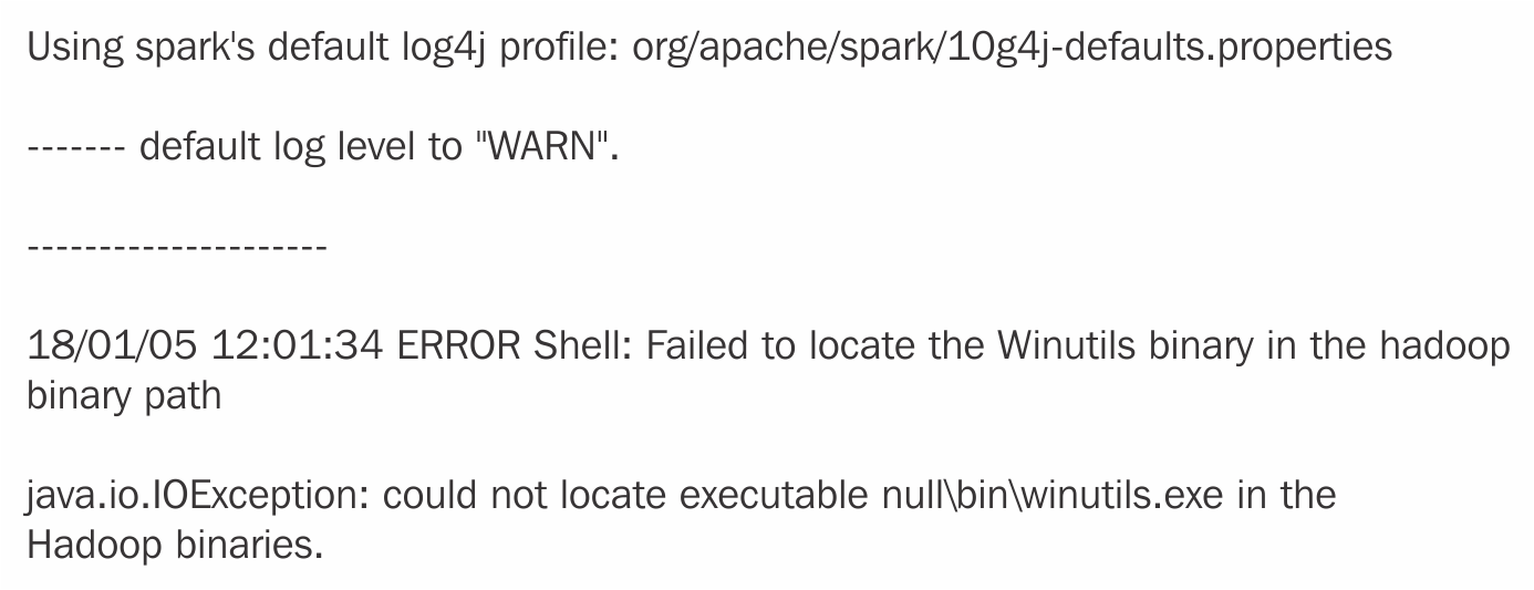
Error message on Windows
To get around this issue, you may proceed with the following steps:
- Create a new folder as
C\tmp\hive. - Then get the missing
WINUTILS.exebinary from here: https://github.com/steveloughran/winutils. Drop this intoC\Hadoop\bin.
The preceding step 2 is necessary because the Spark download does not contain the WINUTILS.exe that is required to run Hadoop. That, then, is the source of the java.io.IOException.
With that knowledge, open up the Command Prompt window in administrator mode and execute the newly downloaded WINUTILS.EXE like this:
winutils.exe chmod -R 777 C:\tmp\hiveNext, issue the spark-shell command. This time around, Spark's interactive development environment launches normally, spinning up its own SparkContext instance sc and a SparkSession spark session, respectively. While the sc feature is a powerful entry point to the underlying local standalone cluster, spark is the main entry point to Spark's data processing APIs.
The following is the output from the spark-shell command.SparkContext is made available to you as sc and the Spark session is available to you as spark:
C:\Users\Ilango\Documents\Packt\DevProjects\Chapter1>spark-shell --master local[2]
Spark context Web UI available at http://192.168.56.1:4040
Spark context available as 'sc' (master = local[2], app id = local-1520484594646).
Spark session available as 'spark'.
Welcome to
 ____ __
 / __/__ ___ _____/ /__
 _\ \/ _ \/ _ `/ __/ '_/
 /___/ .__/\_,_/_/ /_/\_\ version 2.2.1
/_/
Using Scala version 2.11.8 (Java HotSpot(TM) 64-Bit Server VM, Java 1.8.0_102)
Type in expressions to have them evaluated.
Type :help for more information.
scala>
The local[2] option in the spark-shell launch shown earlier lets us run Spark locally with 2 threads.
Before diving into the next topic in this section, it is a good idea to understand the following Spark shell development environment features that make development and data analysis possible:
SparkSessionSparkBuilderSparkContextSparkConf
TheSparkSession API (https://spark.apache.org/docs/2.2.1/api/scala/index.html#org.apache.spark.sql.SparkSession) describes SparkSession as a programmatic access entry point to Spark's dataset and dataframe APIs, respectively.
What is SparkBuilder? The SparkBuilder companion object contains a builder method, which, when invoked, allows us to retrieve an existing SparkSession or even create one. We will now obtain our SparkSession instance in a two-step process, as follows:
- Import the
SparkSessionclass. - Invoke the
buildermethod withgetOrCreateon the resultingbuilder:
scala> import org.apache.spark.sql.SparkSession
import org.apache.spark.sql.SparkSession

scala> lazy val session: SparkSession = SparkSession.builder().getOrCreate()
res7: org.apache.spark.sql.SparkSession = org.apache.spark.sql.SparkSession@6f68756d
The SparkContext API (https://spark.apache.org/docs/2.2.1/api/scala/index.html#org.apache.spark.SparkContext) describes SparkContext as a first-line entry point for setting or configuring Spark cluster properties (RDDs, accumulators, broadcast variables, and much more) affecting the cluster's functionality. One way this configuration happens is by passing in a SparkConf instance as a SparkContext constructor parameter. One SparkContext exists per JVM instance.
In a sense, SparkContext is also how a Spark driver application connects to a cluster through, for example, Hadoop's Yarn ResourceManager (RM).
Let's inspect our Spark environment now. We will start by launching the Spark shell. That said, a typical Spark shell interactive environment screen has its own SparkSession available as spark, whose value we try to read off in the code block as follows:
scala> spark
res21: org.apache.spark.sql.SparkSession = org.apache.spark.sql.SparkSession@6f68756d
The Spark shell also boasts of its own SparkContext instance sc, which is associated with SparkSession spark. In the following code, sc returns SparkContext:
scala> sc
res5: org.apache.spark.SparkContext = org.apache.spark.SparkContext@553ce348
sc can do more. In the following code, invoking the version method on sc gives us the version of Spark running in our cluster:
scala> sc.version
res2: String = 2.2.1
scala> spark
res3: org.apache.spark.sql.SparkSession = org.apache.spark.sql.SparkSession@6f68756d
Since sc represents a connection to the Spark cluster, it holds a special object called SparkConf, holding cluster configuration properties in an Array. Invoking the getConf method on the SparkContext yields SparkConf, whose getAll method (shown as follows) yields an Array of cluster (or connection) properties, as shown in the following code:
scala> sc.getConf.getAll
res17: Array[(String, String)] = Array((spark.driver.port,51576), (spark.debug.maxToStringFields,25), (spark.jars,""), (spark.repl.class.outputDir,C:\Users\Ilango\AppData\Local\Temp\spark-47fee33b-4c60-49d0-93aa-3e3242bee7a3\repl-e5a1acbd-6eb9-4183-8c10-656ac22f71c2), (spark.executor.id,driver), (spark.submit.deployMode,client), (spark.driver.host,192.168.56.1), (spark.app.id,local-1520484594646), (spark.master,local[2]), (spark.home,C:\spark-2.2.1-bin-hadoop2.7\bin\..))
Note
There may be references to sqlContext and sqlContext.implicits._ in the Spark shell. What is sqlContext? As of Spark 2 and the preceding versions, sqlContext is deprecated and SparkSession.builder is used instead to return a SparkSession instance, which we reiterate is the entry point to programming Spark with the dataset and dataframe API. Hence, we are going to ignore those sqlContext instances and focus onSparkSession instead.
Note that spark.app.name bears the default name spark-shell. Let's assign a different name to the app-name property as Iris-Pipeline. We do this by invoking the setAppName method and passing to it the new app name, as follows:
scala> sc.getConf.setAppName("Iris-Pipeline")
res22: org.apache.spark.SparkConf = org.apache.spark.SparkConf@e8ce5b1
To check if the configuration change took effect, let's invoke the getAll method again. The following output should reflect that change. It simply illustrates how SparkContext can be used to modify our cluster environment:
scala> sc.conf.getAll
res20: Array[(String, String)] = Array((spark.driver.port,51576), (spark.app.name,Spark shell), (spark.sql.catalogImplementation,hive), (spark.repl.class.uri,spark://192.168.56.1:51576/classes), (spark.debug.maxToStringFields,150), (spark.jars,""), (spark.repl.class.outputDir,C:\Users\Ilango\AppData\Local\Temp\spark-47fee33b-4c60-49d0-93aa-3e3242bee7a3\repl-e5a1acbd-6eb9-4183-8c10-656ac22f71c2), (spark.executor.id,driver), (spark.submit.deployMode,client), (spark.driver.host,192.168.56.1), (spark.app.id,local-1520484594646), (spark.master,local[2]), (spark.home,C:\spark-2.2.1-bin-hadoop2.7\bin\..))
The spark.app.name property just had its value updated to the new name. Our goal in the next section is to use spark-shell to analyze data in an interactive fashion.
We will develop a simple Scala program in the Spark shell's interactive Scala shell. We will restate our goal, which is that we want to be able to analyze data interactively. That dataset—an externalcomma-separated values (CSV) file called iris.csv—resides in the same folder where spark-shell is launched from.
This program, which could just as well be written in a regular Scala Read Eval Print Loop (REPL) shell, reads a file, and prints out its contents, getting a data analysis task done. However, what is important here is that the Spark shell is flexible in that it also allows you to write Scala code that will allow you to easily connect your data with various Spark APIs and derive abstractions, such as dataframes or RDDs, in some useful way. More about DataFrame and Dataset to follow:
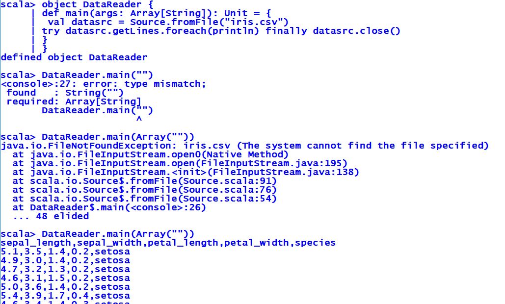
Reading iris.csv with source
In the preceding program, nothing fancy is happening. We are trying to read a file called iris.csv using the Source class. We import the Source.scala file from the scala.io package and from there on, we create an object called DataReader and a main method inside it. Inside the main method, we invoke the fromFile method of the companion object Source. The fromFile method takes in a string representation of the dataset file path as an argument and returns a BufferedSource instance, which we assign to a val that we name datasrc. By the way, the API for Source can be found at https://www.scala-lang.org/api/current/scala/io/Source.html.
On the BufferedSource handle, we then invoke the getLines method that returns an iterator, which in turn invokes foreach that will print out all the lines in iris.csv minus the newline characters. We wrap all of this code in a try and a catch and a finally. The finally construct exists for a reason and that has to do with the fact that we need to close the BufferedSource instance datasrc after it is done working on the file.
Initially, we ran into a FileNotFoundException because the dataset file iris.csv was not found. The CSV file is then dropped in, the program is run, and the output is what we expect.
That wasn't so hard. In the next subsection, the goal is to read our iris.csv file and derive Dataset or DataFrame out of it.
The Spark API for https://spark.apache.org/docs/2.2.1/api/scala/index.html#org.apache.spark.sql.Dataset has it that a DataFrame is Dataset[Row] and that Dataset contains a view called DataFrame. Falling back to the description of Dataset in the Spark documentation, we can redefine Dataset as a Spark abstraction of distributed collections holding data items. That said, Dataset[Row] contains rows. Row could be an abstraction representing a row from the raw file dataset.
We need to read the iris.csv file and transform it into DataFrame. That is the stated goal of this subsection and that is exactly what we shall accomplish very soon.
With all this in mind, lets get down to building DataFrame. We start by invoking the read method on spark, ourSparkSession:
scala> val dfReader1 = spark.read
dfReader1: org.apache.spark.sql.DataFrameReader = org.apache.spark.sql.DataFrameReader@66df362c
The read() invoke produced DataFrameReaderdfReader1, which according to https://spark.apache.org/docs/2.2.1/api/scala/index.html#org.apache.spark.sql.DataFrameReader is an interface to load a dataset from external storage systems.
Next, we will inform Spark that our data is in CSV format. This is done by invoking the format method with a com.databricks.spark.csv argument that Spark recognizes:
scala> val dfReader2 = dfReader1.format("com.databricks.spark.csv")
dfReader2: org.apache.spark.sql.DataFrameReader = org.apache.spark.sql.DataFrameReader@66df362c
The format method simply returned DataFrameReader again. The iris.csv file contains header. We could specify this as an input option:
scala> val dfReader3 = dfReader2.option("header", true)
dfReader3: org.apache.spark.sql.DataFrameReader = org.apache.spark.sql.DataFrameReader@66df362c
That returned our same old DataFrameReader.
What we need next is a way to identify the schema for us. Invoking the option method again with a key inferSchema and a value of true lets Spark infer the schema automatically for us:
scala> val dfReader4 = dfReader3.option("inferSchema",true)
dfReader4: org.apache.spark.sql.DataFrameReader = org.apache.spark.sql.DataFrameReader@66df362c
Let's load our input now:
scala> val dFrame = dfReader4.load("iris.csv")
dFrame: org.apache.spark.sql.DataFrame = [Id: int, SepalLengthCm: double ... 4 more fields]
DataFrameReader transformed our input CSV into DataFrame! This was exactly what we set out to do.
With our DataFrame being a view on Dataset[Row], all the methods on Dataset are available.
For now, we want to see what this dataset has in it. The raw file had 150 columns in it. Therefore, we want Spark to:
- Return the row count in our dataset
- Display the top 20 rows of our dataset
Next, we will invoke the count method. We want to reaffirm the number of rows contained in the dataset:
scala> dFrame.count
res1: Long = 150
We just invoked the count method on our DataFrame. That returned the number 150, which is right.
Next, we will bring together all of the code developed in this section into one line of code:
scala> val irisDataFrame = spark.read.format("com.databricks.spark.csv").option("header",true).option("inferSchema", true).load("iris.csv").show
We just created DataFrameirisDataFrame . If you want to view the DataFrame, just invoke the show method on it. This will return the first 20 rows of the irisDataFrame DataFrame:
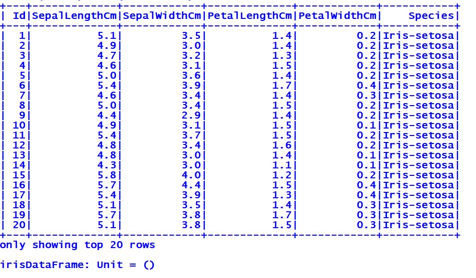
First 20 rows of the Iris dataset
At this point, type :quit or Ctrl + D to exit the Spark shell. This wraps up this section, but opens a segue to the next, where we take things to the next level. Instead of relying on spark-shell to develop a larger program, we will create our Iris prediction pipeline program in an SBT project. This is the focus of the next section.
In this section, we will set forth what our pipeline implementation objectives are. We will document tangible results as we step through individual implementation steps.
Before we implement the Iris pipeline, we want to understand what a pipeline is from a conceptual and practical perspective. Therefore, we define a pipeline as a DataFrame processing workflow with multiple pipeline stages operating in a certain sequence.
A DataFrame is a Spark abstraction that provides an API. This API lets us work with collections of objects. At a high-level it represents a distributed collection holding rows of data, much like a relational database table. Each member of a row (for example, a Sepal-Width measurement) in this DataFrame falls under a named column called Sepal-Width.
Each stage in a pipeline is an algorithm that is either a Transformer or an Estimator. As a DataFrame or DataFrame(s) flow through the pipeline, two types of stages (algorithms) exist:
Transformerstage: This involves a transformation action that transforms oneDataFrameinto anotherDataFrameEstimatorstage: This involves a training action on aDataFramethat produces anotherDataFrame.
In summary, a pipeline is a single unit, requiring stages, but inclusive of parameters and DataFrame(s). The entire pipeline structure is listed as follows:
TransformerEstimatorParameters(hyper or otherwise)DataFrame
This is where Spark comes in. Its MLlib library provides a set of pipeline APIs allowing developers to access multiple algorithms and facilitates their combining into a single pipeline of ordered stages, much like a sequence of choreographed motions in a ballet. In this chapter, we will use the random forest classifier.
We covered essential pipeline concepts. These are practicalities that will help us move into the section, where we will list implementation objectives.
Before listing the implementation objectives, we will lay out an architecture for our pipeline. Shown here under are two diagrams representing an ML workflow, a pipeline.
The following diagrams together help in understanding the different components of this project. That said, this pipeline involves training (fitting), transformation, and validation operations. More than one model is trained and the best model (or mapping function) is selected to give us an accurate approximation predicting the species of an Iris flower (based on measurements of those flowers):

Project block diagram
A breakdown of the project block diagram is as follows:
- Spark, which represents the Spark cluster and its ecosystem
- Training dataset
- Model
- Dataset attributes or feature measurements
- An inference process, that produces a prediction column
The following diagram represents a more detailed description of the different phases in terms of the functions performed in each phase. Later we will come to visualize pipeline in terms of its constituent stages.
For now, the diagram depicts four stages, starting with a data pre-processing phase, which is considered separate from the numbered phases deliberately. Think of the pipeline as a two-step process:
- A data cleansing phase, or pre-processing phase. An important phase that could include a subphase of Exploratory Data Analysis (EDA) (not explicitly depicted in the latter diagram).
- A data analysis phase that begins with Feature Extraction, followed by Model Fitting, and Model validation, all the way to deployment of an Uber pipeline JAR into Spark:

Pipeline diagram
Referring to the preceding diagram, the first implementation objective is to set up Spark inside an SBT project. An SBT project is a self-contained application, which we can run on the command line to predict Iris labels. In the SBT project, dependencies are specified in a build.sbt file and our application code will create its own SparkSession and SparkContext.
So that brings us to a listing of implementation objectives and these are as follows:
- Get the Iris dataset from the UCI Machine Learning Repository
- Conduct preliminary EDA in the Spark shell
- Create a new Scala project in IntelliJ, and carry out all implementation steps, until the evaluation of the Random Forest classifier
- Deploy the application to your local Spark cluster
Head over to the UCI Machine Learning Repository website at https://archive.ics.uci.edu/ml/datasets/iris and click on Download: Data Folder. Extract this folder someplace convenient and copy over iris.csv into the root of your project folder.
You may refer back to the project overview for an in-depth description of the Iris dataset. We depict the contents of the iris.csv file here, as follows:

A snapshot of the Iris dataset with 150 sets
You may recall that the iris.csv file is a 150-row file, with comma-separated values.
Now that we have the dataset, the first step will be performing EDA on it. The Iris dataset is multivariate, meaning there is more than one (independent) variable, so we will carry out a basic multivariate EDA on it. But we need DataFrame to let us do that. How we create a dataframe as a prelude to EDA is the goal of the next section.
Before we get down to building the SBT pipeline project, we will conduct a preliminary EDA in spark-shell. The plan is to derive a dataframe out of the dataset and then calculate basic statistics on it.
We have three tasks at hand for spark-shell:
- Fire up
spark-shell - Load the
iris.csvfile and buildDataFrame - Calculate the statistics
We will then port that code over to a Scala file inside our SBT project.
That said, let's get down to loading the iris.csv file (inputting the data source) before eventually building DataFrame.
Fire up the Spark Shell by issuing the following command on the command line.
spark-shell --master local[2]
In the next step, we start with the available Spark session 'spark'. 'spark' will be our entry point to programming with Spark. It also holds properties required to connect to our Spark (local) cluster. With this information, our next goal is to load the iris.csv file and produce a DataFrame
The first step to loading the iris csv file is to invoke the read method on spark. The read method returns DataFrameReader, which can be used to read our dataset:
val dfReader1 = spark.read
dfReader1: org.apache.spark.sql.DataFrameReader=org.apache.spark.sql.DataFrameReader@6980d3b3
dfReader1 is of type org.apache.spark.sql.DataFrameReader. Calling the format method on dfReader1 with Spark's com.databricks.spark.csv CSV format-specifier string returns DataFrameReader again:
val dfReader2 = dfReader1.format("com.databricks.spark.csv")
dfReader2: org.apache.spark.sql.DataFrameReader=org.apache.spark.sql.DataFrameReader@6980d3b3
After all, iris.csv is a CSV file.
Needless to say, dfReader1 and dfReader2 are the same DataFrameReader instance.
At this point, DataFrameReader needs an input data source option in the form of a key-value pair. Invoke the option method with two arguments, a key "header" of type string and its value true of type Boolean:
val dfReader3 = dfReader2.option("header", true)In the next step, we invoke the option method again with an argument inferSchema and a true value:
val dfReader4 = dfReader3.option("inferSchema", true)What is inferSchema doing here? We are simply telling Spark to guess the schema of our input data source for us.
Up until now, we have been preparing DataFrameReader to load iris.csv. External data sources require a path for Spark to load the data for DataFrameReader to process and spit out DataFrame.
The time is now right to invoke the load method on DataFrameReaderdfReader4. Pass into the load method the path to the Iris dataset file. In this case, the file is right under the root of the project folder:
val dFrame1 = dfReader4.load("iris.csv")
dFrame1: org.apache.spark.sql.DataFrame = [Id: int, SepalLengthCm: double ... 4 more fields]
That's it. We now have DataFrame!
Invoking the describe method on this DataFrame should cause Spark to perform a basic statistical analysis on each column of DataFrame:
dFrame1.describe("Id","SepalLengthCm","SepalWidthCm","PetalLengthCm","PetalWidthCm","Species")
WARN Utils: Truncated the string representation of a plan since it was too large. This behavior can be adjusted by setting 'spark.debug.maxToStringFields' in SparkEnv.conf.
res16: org.apache.spark.sql.DataFrame = [summary: string, Id: string ... 5 more fields]
Lets fix the WARN.Utils issue described in the preceding code block. The fix is to locate the file spark-defaults-template.sh under SPARK_HOME/conf and save it as spark-defaults.sh.
At the bottom of this file, add an entry for spark.debug.maxToStringFields. The following screenshot illustrates this:

Fixing the WARN Utils problem in spark-defaults.sh
Save the file and restart spark-shell.
Now, inspect the updated Spark configuration again. We updated the value of spark.debug.maxToStringFields in the spark-defaults.sh file. This change is supposed to fix the truncation problem reported by Spark. We will confirm imminently that the change we made caused Spark to update its configuration also. That is easily done by inspecting SparkConf.
As before, invoking the getConf returns the SparkContext instance that stores configuration values. Invoking getAll on that instance returns an Array of configuration values. One of those values is an updated value of spark.debug.maxToStringFields:
sc.getConf.getAll
res4: Array[(String, String)] = Array((spark.repl.class.outputDir,C:\Users\Ilango\AppData\Local\Temp\spark-10e24781-9aa8-495c-a8cc-afe121f8252a\repl-c8ccc3f3-62ee-46c7-a1f8-d458019fa05f), (spark.app.name,Spark shell), (spark.sql.catalogImplementation,hive), (spark.driver.port,58009), (spark.debug.maxToStringFields,150),
That updated value for spark.debug.maxToStringFields is now 150.
Run the invoke on the dataframe describe method and pass to it column names:
val dFrame2 =  dFrame1.describe("Id","SepalLengthCm","SepalWidthCm","PetalLengthCm","PetalWidthCm","Species"
)
dFrame2: org.apache.spark.sql.DataFrame = [summary: string, Id: string ... 5 more fields]
The invoke on the describe method of DataFramedfReader results in a transformed DataFrame that we call dFrame2. On dFrame2, we invoke the show method to return a table of statistical results. This completes the first phase of a basic yet important EDA:
val dFrame2Display= = dfReader2.show
The results of the statistical analysis are shown in the following screenshot:

Results of statistical analysis
We did all that extra work simply to demonstrate the individual data reading, loading, and transformation stages. Next, we will wrap all of our previous work in one line of code:
val dfReader = spark.read.format("com.databricks.spark.csv").option("header",true).option("inferSchema",true).load("iris.csv")
dfReader: org.apache.spark.sql.DataFrame = [Id: int, SepalLengthCm: double ... 4 more fields]
That completes the EDA on spark-shell. In the next section, we undertake steps to implement, build (using SBT), deploy (using spark-submit), and execute our Spark pipeline application. We start by creating a skeletal SBT project.
Lay out your SBT project in a folder of your choice and name it IrisPipeline or any name that makes sense to you. This will hold all of our files needed to implement and run the pipeline on the Iris dataset.
The structure of our SBT project looks like the following:

Project structure
We will list dependencies in the build.sbt file. This is going to be an SBT project. Hence, we will bring in the following key libraries:
- Spark Core
- Spark MLlib
- Spark SQL
The following screenshot illustrates the build.sbt file:

The build.sbt file with Spark dependencies
The build.sbt file referenced in the preceding snapshot is readily available for you in the book's download bundle. Drill down to the folder Chapter01 code under ModernScalaProjects_Code and copy the folder over to a convenient location on your computer.
Drop the iris.csv file that you downloaded in Step 1 – getting the Iris dataset from the UCI Machine Learning Repository into the root folder of our new SBT project. Refer to the earlier screenshot that depicts the updated project structure with the iris.csv file inside of it.
Step 4 is broken down into the following steps:
- Create the Scala file
iris.scalain thecom.packt.modern.chapter1package. - Up until now, we relied on
SparkSessionandSparkContext, whichspark-shellgave us. This time around, we need to createSparkSession, which will, in turn, give usSparkContext.
What follows is how the code is laid out in the iris.scala file.
In iris.scala, after the package statement, place the following import statements:
import org.apache.spark.sql.SparkSession
Create SparkSession inside a trait, which we shall call IrisWrapper:
lazy val session: SparkSession = SparkSession.builder().getOrCreate()
Just one SparkSession is made available to all classes extending from IrisWrapper. Create val to hold the iris.csv file path:
val dataSetPath = "<<path to folder containing your iris.csv file>>\\iris.csv"
Create a method to build DataFrame. This method takes in the complete path to the Iris dataset path as String and returns DataFrame:
def buildDataFrame(dataSet: String): DataFrame = {
/*
 The following is an example of a dataSet parameter string: "C:\\Your\\Path\\To\\iris.csv"
*/
Import the DataFrame class by updating the previous import statement for SparkSession:
import org.apache.spark.sql.{DataFrame, SparkSession}Create a nested function inside buildDataFrame to process the raw dataset. Name this function getRows. getRows which takes no parameters but returns Array[(Vector, String)]. The textFile method on the SparkContext variable processes the iris.csv into RDD[String]:
val result1: Array[String] = session.sparkContext.textFile(<<path to iris.csv represented by the dataSetPath variable>>)
The resulting RDD contains two partitions. Each partition, in turn, contains rows of strings separated by a newline character, '\n'. Each row in the RDD represents its original counterpart in the raw data.
In the next step, we will attempt several data transformation steps. We start by applying a flatMap operation over the RDD, culminating in the DataFrame creation. DataFrame is a view over Dataset, which happens to the fundamental data abstraction unit in the Spark 2.0 line.
We will get started by invoking flatMap, by passing a function block to it, and successive transformations listed as follows, eventually resulting in Array[(org.apache.spark.ml.linalg.Vector, String)]. A vector represents a row of feature measurements.
The Scala code to give us Array[(org.apache.spark.ml.linalg.Vector, String)] is as follows:
//Each line in the RDD is a row in the Dataset represented by a String, which we can 'split' along the new //line character
val result2: RDD[String] = result1.flatMap { partition => partition.split("\n").toList }

//the second transformation operation involves a split inside of each line in the dataset where there is a //comma separating each element of that line
val result3: RDD[Array[String]] = result2.map(_.split(","))
Next, drop the header column, but not before doing a collection that returns an Array[Array[String]]:
val result4: Array[Array[String]] = result3.collect.drop(1)
The header column is gone; now import the Vectors class:
import org.apache.spark.ml.linalg.Vectors
Now, transform Array[Array[String]] intoArray[(Vector, String)]:
val result5 = result4.map(row => (Vectors.dense(row(1).toDouble, row(2).toDouble, row(3).toDouble, row(4).toDouble),row(5)))
The last step remaining is to create a final DataFrame
Now, we invoke the createDataFrame method with a parameter, getRows. This returns DataFrame with featureVector and speciesLabel (for example, Iris-setosa):
val dataFrame = spark.createDataFrame(result5).toDF(featureVector, speciesLabel)
Display the top 20 rows in the new dataframe:
dataFrame.show
+--------------------+-------------------------+
|iris-features-column|iris-species-label-column|
+--------------------+-------------------------+
| [5.1,3.5,1.4,0.2]| Iris-setosa|
| [4.9,3.0,1.4,0.2]| Iris-setosa|
| [4.7,3.2,1.3,0.2]| Iris-setosa|
.....................
.....................
+--------------------+-------------------------+
only showing top 20 rows
We need to index the species label column by converting the strings Iris-setosa, Iris-virginica, and Iris-versicolor into doubles. We will use a StringIndexer to do that.
Now create a file called IrisPipeline.scala.
Create an object IrisPipeline that extends our IrisWrapper trait:
object IrisPipeline extends IrisWrapper {Import the StringIndexer algorithm class:
import org.apache.spark.ml.feature.StringIndexer
Now create a StringIndexer algorithm instance. The StringIndexer will map our species label column to an indexed learned column:
val indexer = new StringIndexer().setInputCol
(irisFeatures_CategoryOrSpecies_IndexedLabel._2).setOutputCol(irisFeatures_CategoryOrSpecies_IndexedLabel._3)
Now, let's split our dataset in two by providing a random seed:
val splitDataSet: Array[org.apache.spark.sql.Dataset
[org.apache.spark.sql.Row]] = dataSet.randomSplit(Array(0.85, 0.15), 98765L)
Now our new splitDataset contains two datasets:
- Train dataset: A dataset containing
Array[(Vector, iris-species-label-column: String)] - Test dataset: A dataset containing
Array[(Vector, iris-species-label-column: String)]
Confirm that the new dataset is of size 2:
splitDataset.size
res48: Int = 2
Assign the training dataset to a variable, trainSet:
val trainDataSet = splitDataSet(0)
trainSet: org.apache.spark.sql.Dataset[org.apache.spark.sql.Row] = [iris-features-column: vector, iris-species-label-column: string]
Assign the testing dataset to a variable, testSet:
val testDataSet = splitDataSet(1)
testSet: org.apache.spark.sql.Dataset[org.apache.spark.sql.Row] = [iris-features-column: vector, iris-species-label-column: string]
Count the number of rows in the training dataset:
trainSet.count
res12: Long = 14
Count the number of rows in the testing dataset:
testSet.count
res9: Long = 136
There are 150 rows in all.
In reference to Step 5 - DataFrame Creation. This DataFrame 'dataFrame' contains column names that corresponds to the columns present in the DataFrame produced in that step
The first step to create a classifier is to pass into it (hyper) parameters. A fairly comprehensive list of parameters look like this:
- From 'dataFrame' we need the Features column name - iris-features-column
- From 'dataFrame' we also need the Indexed label column name - iris-species-label-column
- The
sqrtsetting forfeatureSubsetStrategy - Number of features to be considered per split (we have 150 observations and four features that will make our
max_featuresvalue2) - Impurity settings—values can be gini and entropy
- Number of trees to train (since the number of trees is greater than one, we set a tree maximum depth), which is a number equal to the number of nodes
- The required minimum number of feature measurements (sampled observations), also known as the minimum instances per node
Look at the IrisPipeline.scala file for values of each of these parameters.
But this time, we will employ an exhaustive grid search-based model selection process based on combinations of parameters, where parameter value ranges are specified.
Create a randomForestClassifier instance. Set the features and featureSubsetStrategy:
val randomForestClassifier = new RandomForestClassifier()
  .setFeaturesCol(irisFeatures_CategoryOrSpecies_IndexedLabel._1)
  .setFeatureSubsetStrategy("sqrt")
Start building Pipeline, which has two stages, Indexer and Classifier:
val irisPipeline = new Pipeline().setStages(Array[PipelineStage](indexer) ++ Array[PipelineStage](randomForestClassifier))
Next, set the hyperparameter num_trees (number of trees) on the classifier to 15, a Max_Depth parameter, and an impurity with two possible values of gini and entropy.
Build a parameter grid with all three hyperparameters:
val finalParamGrid: Array[ParamMap] = gridBuilder3.build()
Next, we want to split our training set into a validation set and a training set:
val validatedTestResults: DataFrame = new TrainValidationSplit()
On this variable, set Seed, set EstimatorParamMaps, set Estimator with irisPipeline, and set a training ratio to 0.8:
val validatedTestResults: DataFrame = new TrainValidationSplit().setSeed(1234567L).setEstimator(irisPipeline)
Finally, do a fit and a transform with our training dataset and testing dataset. Great! Now the classifier is trained. In the next step, we will apply this classifier to testing the data.
The purpose of our validation set is to be able to make a choice between models. We want an evaluation metric and hyperparameter tuning. We will now create an instance of a validation estimator called TrainValidationSplit, which will split the training set into a validation set and a training set:
val validatedTestResults.setEvaluator(new MulticlassClassificationEvaluator())
Next, we fit this estimator over the training dataset to produce a model and a transformer that we will use to transform our testing dataset. Finally, we perform a validation for hyperparameter tuning by applying an evaluator for a metric.
The new ValidatedTestResultsDataFrame should look something like this:
--------+
 |iris-features-column|iris-species-column|label| rawPrediction| probability|prediction|
 +--------------------+-------------------+-----+--------------------+
 | [4.4,3.2,1.3,0.2]| Iris-setosa| 0.0| [40.0,0.0,0.0]| [1.0,0.0,0.0]| 0.0|
 | [5.4,3.9,1.3,0.4]| Iris-setosa| 0.0| [40.0,0.0,0.0]| [1.0,0.0,0.0]| 0.0|
 | [5.4,3.9,1.7,0.4]| Iris-setosa| 0.0| [40.0,0.0,0.0]| [1.0,0.0,0.0]| 0.0|
Let's return a new dataset by passing in column expressions for prediction and label:
val validatedTestResultsDataset:DataFrame = validatedTestResults.select("prediction", "label")In the line of code, we produced a new DataFrame with two columns:
- An input label
- A predicted label, which is compared with its corresponding value in the input label column
That brings us to the next step, an evaluation step. We want to know how well our model performed. That is the goal of the next step.
In this section, we will test the accuracy of the model. We want to know how well our model performed. Any ML process is incomplete without an evaluation of the classifier.
That said, we perform an evaluation as a two-step process:
- Evaluate the model output
- Pass in three hyperparameters:
val modelOutputAccuracy: Double = new MulticlassClassificationEvaluator()
Set the label column, a metric name, the prediction column label, and invoke evaluation with the validatedTestResults dataset.
Note the accuracy of the model output results on the testing dataset from the modelOutputAccuracy variable.
The other metrics to evaluate are how close the predicted label value in the 'predicted' column is to the actual label value in the (indexed) label column.
Next, we want to extract the metrics:
val multiClassMetrics = new MulticlassMetrics(validatedRDD2)
Our pipeline produced predictions. As with any prediction, we need to have a healthy degree of skepticism. Naturally, we want a sense of how our engineered prediction process performed. The algorithm did all the heavy lifting for us in this regard. That said, everything we did in this step was done for the purpose of evaluation. Who is being evaluated here or what evaluation is worth reiterating? That said, we wanted to know how close the predicted values were compared to the actual label value. To obtain that knowledge, we decided to use the MulticlassMetrics class to evaluate metrics that will give us a measure of the performance of the model via two methods:
- Accuracy
- Weighted precision
The following lines of code will give us value of Accuracy and Weighted Precision. First we will create an accuracyMetrics tuple, which should contain the values of both accuracy and weighted precision
val accuracyMetrics = (multiClassMetrics.accuracy, multiClassMetrics.weightedPrecision)
Obtain the value of accuracy.
val accuracy = accuracyMetrics._1
Next, obtain the value of weighted precision.
val weightedPrecsion = accuracyMetrics._2
These metrics represent evaluation results for our classifier or classification model. In the next step, we will run the application as a packaged SBT application.
At the root of your project folder, issue the sbt console command, and in the Scala shell, import the IrisPipeline object and then invoke the main method of IrisPipeline with the argument iris:
sbt console
scala>
import com.packt.modern.chapter1.IrisPipeline
IrisPipeline.main(Array("iris")
Accuracy (precision) is 0.9285714285714286 Weighted Precision is: 0.9428571428571428
In the next section, we will show you how to package the application so that it is ready to be deployed into Spark as an Uber JAR.
In the root folder of your SBT application, run:
sbt packageWhen SBT is done packaging, the Uber JAR can be deployed into our cluster, using spark-submit, but since we are in standalone deploy mode, it will be deployed into [local]:

The application JAR file
The package command created a JAR file that is available under the target folder. In the next section, we will deploy the application into Spark.
At the root of the application folder, issue the spark-submit command with the class and JAR file path arguments, respectively.
If everything went well, the application does the following:
- Loads up the data.
- Performs EDA.
- Creates training, testing, and validation datasets.
- Creates a Random Forest classifier model.
- Trains the model.
- Tests the accuracy of the model. This is the most important part—the ML classification task.
- To accomplish this, we apply our trained Random Forest classifier model to the test dataset. This dataset consists of Iris flower data of so far not seen by the model. Unseen data is nothing but Iris flowers picked in the wild.
- Applying the model to the test dataset results in a prediction about the species of an unseen (new) flower.
- The last part is where the pipeline runs an evaluation process, which essentially is about checking if the model reports the correct species.
- Lastly, pipeline reports back on how important a certain feature of the Iris flower turned out to be. As a matter of fact, the petal width turns out to be more important than the sepal width in carrying out the classification task.
That brings us to the last section of this chapter. We will summarize what we have learned. Not only that, we will give readers a glimpse into what they will learn in the next chapter.
In this chapter, we implemented an ML workflow or an ML pipeline. The pipeline combined several stages of data analysis into one workflow. We started by loading the data and from there on, we created training and test data, preprocessed the dataset, trained the RandomForestClassifier model, applied the Random Forest classifier to test data, evaluated the classifier, and computed a process that demonstrated the importance of each feature in the classification. We fulfilled the goal that we laid out early on in the Project overview – problem formulation section.
In the next chapter, we will analyze the Wisconsin Breast Cancer Data Set. This dataset has only categorical data. We will build another pipeline, but this time, we will set up the Hortonworks Development Platform Sandbox to develop and deploy a breast cancer prediction pipeline. Given a set of categorical feature variables, this pipeline will predict whether a given sample is benign or malignant. In the next and the last section of the current chapter, we will list a set of questions that will test your knowledge of what you have learned so far.
Here are a list of questions for your reference:
- What do you understand by EDA? Why is it important?
- Why do we create training and test data?
- Why did we index the data that we pulled from the UCI Machine Learning Repository?
- Why is the Iris dataset so famous?
- Name one powerful feature of the random forest classifier.
- What is supervisory as opposed to unsupervised learning?
- Explain briefly the process of creating our model with training data.
- What are feature variables in relation to the Iris dataset?
- What is the entry point to programming with Spark?
Task: The Iris dataset problem was a statistical classification problem. Create a confusion or error matrix with the rows being predicted setosa, predicted versicolor, and predicted virginica, and the columns being actual species, such as setosa, versicolor, and virginica. Having done that, interpret this matrix.
