Basic plotting

The standard plotting function is plot. Calling plot(x,y) creates a figure window with a plot of y as a function of x. The input arguments are arrays (or lists) of equal length. It is also possible to use plot(y), in which case the values in y will be plotted against their index, that is, plot(y) is a short form of plot(range(len(y)),y).

Here is an example that shows how to plot sin(x) for x ϵ [-2π, 2π]  using 200 sample points and sets markers at every fourth point:

# plot sin(x) for some interval
x = linspace(-2*pi,2*pi,200)
plot(x,sin(x))

# plot marker for every 4th point
samples = x[::4]
plot(samples,sin(samples),'r*')

# add title and grid lines
title('Function sin(x) and some points plotted')
grid()

The result is shown in the following figure (Figure 6.1):

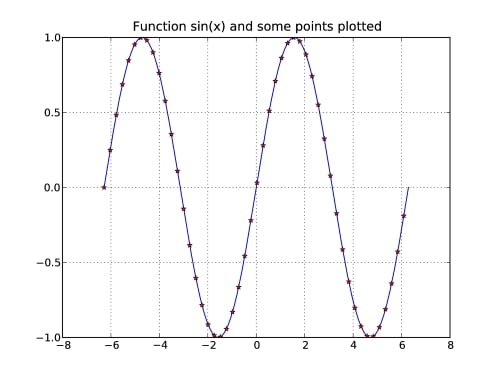
Figure 6.1: A plot of the function sin(x) with grid lines shown.

As you can see, the standard plot is a solid blue curve. Each axis gets automatically scaled to fit...