Download code from GitHub
Reading Time Series Data from Files
In this chapter, we will use pandas, a popular Python library with a rich set of I/O tools, data wrangling, and date/time functionality to streamline working with time series data. In addition, you will explore several reader functions available in pandas to ingest data from different file types, such as Comma-Separated Value (CSV), Excel, and SAS. You will explore reading from files, whether they are stored locally on your drive or remotely on the cloud, such as an AWS S3 bucket.
Time series data is complex and can be in different shapes and formats. Conveniently, the pandas reader functions offer a vast number of arguments (parameters) to help handle such variety in the data.
The pandas library provides two fundamental data structures, Series and DataFrame, implemented as classes. The DataFrame class is a distinct data structure for working with tabular data (think rows and columns in a spreadsheet). The main difference between the two data structures is that a Series is one-dimensional (single column), and a DataFrame is two-dimensional (multiple columns). The relationship between the two is that you get a Series when you slice out a column from a DataFrame. You can think of a DataFrame as a side-by-side concatenation of two or more Series objects.
A particular feature of the Series and DataFrames data structures is that they both have a labeled axis called index. A specific type of index that you will often see with time series data is the DatetimeIndex which you will explore further in this chapter. Generally, the index makes slicing and dicing operations very intuitive. For example, to make a DataFrame ready for time series analysis, you will learn how to create DataFrames with an index of type DatetimeIndex.
We will cover the following recipes on how to ingest data into a pandas DataFrame:
- Reading data from CSVs and other delimited files
- Reading data from an Excel file
- Reading data from URLs
- Reading data from a SAS dataset
Why DatetimeIndex?
A pandas DataFrame with an index of type
DatetimeIndexunlocks a large set of features and useful functions needed when working with time series data. You can think of it as adding a layer of intelligence or awareness to pandas to treat the DataFrame as a time series DataFrame.
Technical requirements
In this chapter and forward, we will be using pandas 1.4.2 (released April 2, 2022) extensively.
Throughout our journey, you will be installing additional Python libraries to use in conjunction with pandas. You can download the Jupyter notebooks from the GitHub repository (https://github.com/PacktPublishing/Time-Series-Analysis-with-Python-Cookbook./blob/main/code/Ch2/Chapter%202.ipynb) to follow along.
You can download the datasets used in this chapter from the GitHub repository using this link: https://github.com/PacktPublishing/Time-Series-Analysis-with-Python-Cookbook./tree/main/datasets/Ch2.
Reading data from CSVs and other delimited files
In this recipe, you will use the pandas.read_csv() function, which offers a large set of parameters that you will explore to ensure the data is properly read into a time series DataFrame. In addition, you will learn how to specify an index column, parse the index to be of the type DatetimeIndex, and parse string columns that contain dates into datetime objects.
Generally, using Python, data read from a CSV file will be in string format (text). When using the read_csv method in pandas, it will try and infer the appropriate data types (dtype), and, in most cases, it does a great job at that. However, there are situations where you will need to explicitly indicate which columns to cast to a specific data type. For example, you will specify which column(s) to parse as dates using the parse_dates parameter in this recipe.
Getting ready
You will be reading a CSV file that contains hypothetical box office numbers for a movie. The file is provided in the GitHub repository for this book. The data file is in datasets/Ch2/movieboxoffice.csv.
How to do it…
You will ingest our CSV file using pandas and leverage some of the available parameters in read_csv:
- First, let's load the libraries:
import pandas as pd
from pathlib import Path
- Create a
Pathobject for the file location:filepath =\ Path('../../datasets/Ch2/movieboxoffice.csv') - Read the CSV file into a DataFrame using the
read_csvfunction and passing thefilepathwith additional parameters.
The first column in the CSV file contains movie release dates, and it needs to be set as an index of type DatetimeIndex (index_col=0 and parse_dates=['Date']). Specify which columns you want to include by providing a list of column names to usecols. The default behavior is that the first row includes the header (header=0):
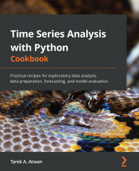
ts = pd.read_csv(filepath,
                 header=0,
                 parse_dates=['Date'],
                 index_col=0,
                 infer_datetime_format=True,
                 usecols=['Date',
                          'DOW',
                          'Daily',
                          'Forecast',
                          'Percent Diff'])
ts.head(5)
This will output the following first five rows:
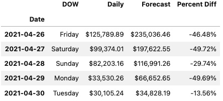
Figure 2.1 – The first five rows of the ts DataFrame using JupyterLab
- Print a summary of the DataFrame to check the index and column data types:
ts.info()
>> <class 'pandas.core.frame.DataFrame'>
DatetimeIndex: 128 entries, 2021-04-26 to 2021-08-31
Data columns (total 4 columns):
 #   Column        Non-Null Count  Dtype
---  ------        --------------  -----
 0   DOW           128 non-null    object
 1   Daily         128 non-null    object
 2   Forecast      128 non-null    object
 3   Percent Diff  128 non-null    object
dtypes: object(4)
memory usage: 5.0+ KB
- Notice that the
Datecolumn is now an index (not a column) of typeDatetimeIndex. Additionally, bothDailyandForecastcolumns have the wrong dtype inference. You would expect them to be of typefloat. The issue is due to the source CSV file containing dollar signs ($) and thousand separators (,) in both columns. The presence of non-numeric characters will cause the columns to be interpreted as strings. A column with thedtypeobject indicates either a string column or a column with mixed dtypes (not homogeneous).
To fix this, you need to remove both the dollar sign ($) and thousand separators (,) or any non-numeric character. You can accomplish this using str.replace(), which can take a regular expression to remove all non-numeric characters but exclude the period (.) for the decimal place. Removing these characters does not convert the dtype, so you will need to cast those two columns as a float dtype using .astype(float):
clean = lambda x: x.str.replace('[^\d]','', regex=True)
c_df = ts[['Daily', 'Forecast']].apply(clean, axis=1)
ts[['Daily', 'Forecast']] = c_df.astype(float)
Print a summary of the updated DataFrame:
ts.info()
>> <class 'pandas.core.frame.DataFrame'>
DatetimeIndex: 128 entries, 2021-04-26 to 2021-08-31
Data columns (total 4 columns):
 #   Column        Non-Null Count  Dtype
---  ------        --------------  -----
 0   DOW           128 non-null    object
 1   Daily         128 non-null    float64
 2   Forecast      128 non-null    float64
 3   Percent Diff  128 non-null    object
dtypes: float64(2), object(2)
memory usage: 5.0+ KB
Now, you have a DataFrame with DatetimeIndex and both Daily and Forecast columns are of dtype float64 (numeric fields).
How it works…
Using pandas for data transformation is fast since it loads the data into memory. For example, the read_csv method reads and loads the entire data into a DataFrame in memory. When requesting a DataFrame summary with the info() method, in addition to column and index data types, the output will display memory usage for the entire DataFrame. To get the exact memory usage for each column, including the index, you can use the memory_usage() method:
ts.memory_usage()
>>
Index           1024
DOW             1024
Daily           1024
Forecast        1024
Percent Diff    1024
dtype: int64
The total will match what was provided in the DataFrame summary:
ts.memory_usage().sum()
>> 5120
So far, you have used a few of the available parameters when reading a CSV file using read_csv. The more familiar you become with the different options available in any of the pandas reader functions, the more upfront preprocessing you can do during data ingestion (reading).
You leveraged the built-in parse_dates argument, which takes in a list of columns (either specified by name or position).The combination of index_col=0 and parse_dates=[0] produced a DataFrame with an index of type DatetimeIndex.
Let's inspect the parameters used in this recipe as defined in the official pandas.read_csv() documentation (https://pandas.pydata.org/pandas-docs/stable/reference/api/pandas.read_csv.html):
filepath_or_buffer: This is the first positional argument and the only required field needed (at a minimum) to read a CSV file. Here, you passed the Python path object namedfilepath. This can also be a string that represents a valid file path such as'../../datasets/Ch2/movieboxoffice.csv'or a URL that points to a remote file location, such as an AWS S3 bucket (we will examine this later in the Reading data from URLs recipe in this chapter).sep: This takes a string to specify which delimiter to use. The default is a comma delimiter (,) which assumes a CSV file. If the file is separated by another delimiter, such as a pipe (|) or semicolon (;), then the argument can be updated, such assep="|" or sep=";".
Another alias to sep is delimiter, which can be used as well as a parameter name.
header: In this case, you specified that the firstrow(0) value contains the header information. The default value isinfer, which usually works as-is in most cases. If the CSV does not contain a header, then you specifyheader=None. If the CSV has a header but you prefer to supply custom column names, then you need to specifyheader=0and overwrite it by providing a list of new column names to thenamesargument.
Recall that you specified which columns to include by passing a list of column names to the usecols parameter. These names are based on the file header (the first row of the CSV file).
If you decide to provide custom header names, you cannot reference the original names in the usecols parameter; this will produce the following error: ValueError: Usecols do not match columns.
parse_dates: In the recipe, you provided a list of column positions using[0], which specified only the first column (by position) should be parsed. Theparse_datesargument can take a list of column names, such as["Date"], or a list of column positions, such as[0, 3], indicating the first and the fourth columns. If you only intend to parse the index column(s) specified in theindex_colparameter, you only need to passTrue(Boolean).index_col: Here, you specified that the first column by position (index_col=0) will be used as the DataFrame index. Alternatively, you could provide the column name as a string (index_col='Date'). The parameter also takes in a list of integers (positional indices) or strings (column names), which would create aMultiIndexobject.usecols: The default value isNone, which includes all the columns in the dataset. Limiting the number of columns to only those that are required results in faster parsing and overall lower memory usage, since you only bring in what is needed. Theusecolsarguments can take a list of column names, such as['Date', 'DOW', 'Daily', 'Percent Diff', 'Forecast']or a list of positional indices, such as[0, 1, 3, 7, 6], which would produce the same result.
There's more…
There are situations where parse_dates may not work (it just cannot parse the date). In such cases, the column(s) will be returned unchanged, and no error will be thrown. This is where the date_parser parameter can be useful.
For example, you can pass a lambda function that uses the to_datetime function in pandas to date_parser. You can specify the string representation for the date format inside to_datetime(), as demonstrated in the following code:
date_parser =lambda x: pd.to_datetime(x, format="%d-%b-%y")
ts = pd.read_csv(filepath,
                 parse_dates=[0],
                 index_col=0,
                 date_parser=date_parser,
                 usecols=[0,1,3, 7, 6])
ts.head()
The preceding code will print out the first five rows of the ts DataFrame displaying a properly parsed Date index.
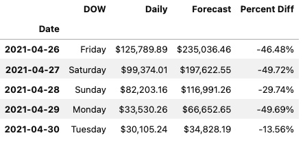
Figure 2.2 – The first five rows of the ts DataFrame using JupyterLab
Let's break it down. In the preceding code, you passed two arguments to the to_datetime function: the object to convert to datetime and an explicit format string. Since the date is stored as a string in the form 26-Apr-21, you passed "%d-%b-%y" to reflect that:
%drepresents the day of the month, such as01or02.%brepresents the abbreviated month name, such asAprorMay.%yrepresents a two-digit year, such as19or20.
Other common string codes include the following:
%Yrepresents the year as a four-digit number, such as2020or2021.%Brepresents the month's full name, such asJanuaryorFebruary.%mrepresents the month as a two-digit number, such as01or02.
For more information on Python's string formats for representing dates, visit https://strftime.org.
See also
According to the pandas documentation, the infer_datetime_format parameter in read_csv() function can speed up the parsing by 5–10x. This is how you can add this to our original script:
ts = pd.read_csv(filepath,
                 header=0,
                 parse_dates=[0],
                 index_col=0,
                 infer_datetime_format= True,
                 usecols=['Date',
                          'DOW',
                          'Daily',
                          'Forecast',
                          'Percent Diff'])
Note that given the dataset is small, the speed improvement may be insignificant.
For more information, please refer to the pandas.read_csv documentation: https://pandas.pydata.org/docs/reference/api/pandas.read_csv.html.
Reading data from an Excel file
To read data from an Excel file, you will need to use a different reader function from pandas. Generally, working with Excel files can be a challenge since the file can contain formatted multi-line headers, merged header cells, and images. They may also contain multiple worksheets with custom names (labels). Therefore, it is vital that you always inspect the Excel file first. The most common scenario is reading from an Excel file that contains data partitioned into multiple sheets, which is the focus of this recipe.
In this recipe, you will be using the pandas.read_excel() function and examining the various parameters available to ensure the data is read properly as a DataFrame with a DatetimeIndex for time series analysis. In addition, you will explore different options to read Excel files with multiple sheets.
Getting ready
To use pandas.read_excel(), you will need to install an additional library for reading and writing Excel files. In the read_excel() function, you will use the engine parameter to specify which library (engine) to use for processing an Excel file. Depending on the Excel file extension you are working with (for example, .xls or .xlsx), you may need to specify a different engine that may require installing an additional library.
The supported libraries (engines) for reading and writing Excel include xlrd, openpyxl, odf, and pyxlsb. When working with Excel files, the two most common libraries are usually xlrd and openpyxl.
The xlrd library only supports .xls files. So, if you are working with an older Excel format, such as .xls, then xlrd will do just fine. For newer Excel formats, such as .xlsx, we will need a different engine, and in this case, openpyxl would be the recommendation to go with.
To install openpyxl using conda, run the following command in the terminal:
>>> conda install openpyxl
To install using pip, run the following command:
>>> pip install openpyxl
We will be using the sales_trx_data.xlsx file, which you can download from the book's GitHub repository. See the Technical requirements section of this chapter. The file contains sales data split by year into two sheets (2017 and 2018), respectively.
How to do it…
You will ingest the Excel file (.xlsx) using pandas and openpyxl, and leverage some of the available parameters in read_excel():
- Import the libraries for this recipe:
import pandas as pd from pathlib import Path filepath = \ Path('../../datasets/Ch2/sales_trx_data.xlsx') - Read the Excel (
.xlxs) file using theread_excel()function. By default, pandas will only read from the first sheet. This is specified under thesheet_nameparameter, which is set to0as the default value. Before passing a new argument, you can usepandas.ExcelFilefirst to inspect the file and determine the number of sheets available. TheExcelFileclass will provide additional methods and properties, such assheet_name, which returns a list of sheet names:excelfile = pd.ExcelFile(filepath) excelfile.sheet_names >> ['2017', '2018']
If you have multiple sheets, you can specify which sheets you want to ingest by passing a list to the sheet_name parameter in read_excel. The list can either be positional arguments, such as first, second, and fifth sheets with [0, 1, 4], sheet names with ["Sheet1", "Sheet2", "Sheet5"], or a combination of both, such as first sheet, second sheet, and a sheet named "Revenue" [0, 1, "Revenue"].
In the following code, you will use sheet positions to read both the first and second sheets (0 and 1 indexes). This will return a Python dictionary object with two DataFrames. Notet hat the returned dictionary (key-value pair) has numeric keys (0 and 1) representing the first and second sheets (positional index), respectively:
ts = pd.read_excel(filepath,
                   engine='openpyxl',
                   index_col=1,
                   sheet_name=[0,1],
                   parse_dates=True)
ts.keys()
>> dict_keys([0, 1])
- Alternatively, you can pass a list of sheet names. Notice that the returned dictionary keys are now strings and represent the sheet names as shown in the following code:
ts = pd.read_excel(filepath,
                   engine='openpyxl',
                   index_col=1,
                   sheet_name=['2017','2018'],
                   parse_dates=True)
ts.keys()
>> dict_keys(['2017', '2018'])
- If you want to read from all the available sheets, you will pass
Noneinstead. The keys for the dictionary, in this case, will represent sheet names:ts = pd.read_excel(filepath, engine='openpyxl', index_col=1, sheet_name=None, parse_dates=True) ts.keys() >> dict_keys(['2017', '2018'])
The two DataFrames within the dictionary are identical (homogeneous-typed) in terms of their schema (column names and data types). You can inspect each DataFrame with ts['2017'].info() and ts['2018'].info().
They both have a DatetimeIndex object, which you specified in the index_col parameter. The 2017 DataFrame consists of 36,764 rows and the 2018 DataFrame consists of 37,360. In this scenario, you want to stack (combine) the two (think UNION in SQL) into a single DataFrame that contains all 74,124 rows and a DatetimeIndex that spans from 2017-01-01 to 2018-12-31.
To combine the two DataFrames along the index axis (stacked one on top of the other), you will use the pandas.concat() function. The default behavior of the concat() function is to concatenate along the index axis (axis=0). In the following code, you will explicitly specify which DataFrames to concatenate:
ts_combined = pd.concat([ts['2017'],ts['2018']])
ts_combined.info()
>> <class 'pandas.core.frame.DataFrame'>
DatetimeIndex: 74124 entries, 2017-01-01 to 2018-12-31
Data columns (total 4 columns):
 #   Column              Non-Null Count  Dtype
---  ------              --------------  -----
 0   Line_Item_ID        74124 non-null  int64
 1   Credit_Card_Number  74124 non-null  int64
 2   Quantity            74124 non-null  int64
 3   Menu_Item           74124 non-null  object
dtypes: int64(3), object(1)
memory usage: 2.8+ MB
- When you have multiple DataFrames returned (think multiple sheets), you can use the
concat()function on the returned dictionary. In other words, you can combine theconcat()andread_excel()functions in one statement. In this case, you will end up with aMultiIndexDataFrame where the first level is the sheet name (or number) and the second level is theDatetimeIndex. For example, using thetsdictionary, you will get a two-level index:MultiIndex([('2017', '2017-01-01'), ..., ('2018', '2018-12-31')], names=[None, 'Date'], length=74124).
To reduce the number of levels, you can use the droplevel(level=0) method to drop the first level after pandas .concat() shown as follows:
ts_combined = pd.concat(ts).droplevel(level=0)
- If you are only reading one sheet, the behavior is slightly different. By default,
sheet_nameis set to0, which means it reads the first sheet. You can modify this and pass a different value (single value), either the sheet name (string) or sheet position (integer). When passing a single value, the returned object will be a pandas DataFrame and not a dictionary:ts = pd.read_excel(filepath, index_col=1, sheet_name='2018', parse_dates=True) type(ts) >> pandas.core.frame.DataFrame
Do note though that if you pass a single value inside two brackets ([1]), then pandas will interpret this differently and the returned object will be a dictionary that contains one DataFrame.
Lastly, note that you did not need to specify the engine in the last example. The read_csv function will determine which engine to use based on the file extension. So, for example, suppose the library for that engine is not installed. In that case, it will throw an ImportError message, indicating that the library (dependency) is missing.
How it works…
The pandas.read_excel() function has many common parameters with the pandas.read_csv() function that you used earlier. The read_excel function can either return a DataFrame object or a dictionary of DataFrames. The dependency here is whether you are passing a single value (scalar) or a list to sheet_name.
In the sales_trx_data.xlsx file, both sheets had the same schema (homogeneous- typed). The sales data was partitioned (split) by year, where each sheet contained sales for a particular year. In this case, concatenating the two DataFrames was a natural choice. The pandas.concat() function is like the DataFrame.append() function, in which the second DataFrame was added (appended) to the end of the first DataFrame. This should be similar in behavior to the UNION clause for those coming from a SQL background.
There's more…
An alternative method to reading an Excel file is with the pandas.ExcelFile() class, which returns a pandas ExcelFile object. Earlier in this recipe, you used ExcelFile() to inspect the number of sheets in the Excel file through the sheet_name property.
The ExcelFile class has several useful methods, including the parse() method to parse the Excel file into a DataFrame, similar to the pandas.read_excel() function.
In the following example, you will use the ExcelFile class to parse the first sheet, assign the first column as an index, and print the first five rows:
excelfile = pd.ExcelFile(filepath)
excelfile.parse(sheet_name='2017',
                index_col=1,
                parse_dates=True).head()
You should see similar results for the first five rows of the DataFrame:
Figure 2.3 – The first five rows of the DataFrame using JupyterLab
From Figure 2.3, it should become clear that ExcelFile.parse() is equivalent to pandas.read_excel().
See also
For more information on pandas.read_excel() and pandas.ExcelFile(), please refer to the official documentation:
- pandas.read_excel(): https://pandas.pydata.org/docs/reference/api/pandas.read_excel.html
- pandas.ExcelFile.parse(): https://pandas.pydata.org/docs/reference/api/pandas.ExcelFile.parse.html
Reading data from URLs
Files can be downloaded and stored locally on your machine, or stored on a remote server or cloud location. In the earlier two recipes, Reading from CSVs and other delimited files, and Reading data from an Excel file, both files were stored locally.
Many of the pandas reader functions can read data from remote locations by passing a URL path. For example, both read_csv() and read_excel() can take a URL to read a file that is accessible via the internet. In this recipe, you will read a CSV file using pandas.read_csv() and Excel files using pandas.read_excel() from remote locations, such as GitHub and AWS S3 (private and public buckets). You will also read data directly from an HTML page into a pandas DataFrame.
Getting ready
You will need to install the AWS SDK for Python (Boto3) for reading files from S3 buckets. Additionally, you will learn how to use the storage_options parameter available in many of the reader functions in pandas to read from S3 without the Boto3 library.
To use an S3 URL (for example, s3://bucket_name/path-to-file) in pandas, you will need to install the s3fs library. You will also need to install an HTML parser for when we use read_html(). For example, for the parsing engine (the HTML parser), you can install either lxml or html5lib; pandas will pick whichever is installed (it will first look for lxml, and if that fails, then for html5lib). If you plan to use html5lib you will need to install Beautiful Soup (beautifulsoup4).
To install using pip, you can use the following command:
>>> pip install boto3 s3fs lxml
To install using Conda, you can use:
>>> conda install boto3 s3fs lxml -y
How to do it…
This recipe will present you with different scenarios when reading data from online (remote) sources. Let's import pandas upfront since you will be using it throughout this recipe:
import pandas as pd
Reading data from GitHub
Sometimes, you may find useful public data on GitHub that you want to use and read directly (without downloading). One of the most common file formats on GitHub are CSV files. Let's start with the following steps:
- To read a CSV file from GitHub, you will need the URL to the raw content. If you copy the file's GitHub URL from the browser and use it as the file path, you will get a URL that looks like this: https://github.com/PacktPublishing/Time-Series-Analysis-with-Python-Cookbook./blob/main/datasets/Ch2/AirQualityUCI.csv. This URL is a pointer to the web page in GitHub and not the data itself; hence when using
pd.read_csv(), it will throw an error:url = 'https://github.com/PacktPublishing/Time-Series-Analysis-with-Python-Cookbook./blob/main/datasets/Ch2/AirQualityUCI.csv' pd.read_csv(url) ParserError: Error tokenizing data. C error: Expected 1 fields in line 62, saw 2
- Instead, you will need the raw content, which will give you a URL that looks like this: https://raw.githubusercontent.com/PacktPublishing/Time-Series-Analysis-with-Python-Cookbook./main/datasets/Ch2/AirQualityUCI.csv:
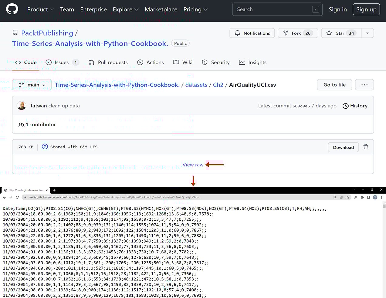
Figure 2.4 – The GitHub page for the CSV file. Note the View raw button
- In Figure 2.4, notice that the values are not comma-separated (not a comma-delimited file); instead, the file uses semicolon (
;) to separate the values.
The first column in the file is the Date column. You will need to parse (parse_date parameter) and convert it to DatetimeIndex (index_col parameter).
Pass the new URL to pandas.read_csv():
url = 'https://media.githubusercontent.com/media/PacktPublishing/Time-Series-Analysis-with-Python-Cookbook./main/datasets/Ch2/AirQualityUCI.csv'
date_parser = lambda x: pd.to_datetime(x, format="%d/%m/%Y")
df = pd.read_csv(url,
                 delimiter=';',
                 index_col='Date',
                 date_parser=date_parser)
df.iloc[:3,1:4]
>>
            CO(GT)  PT08.S1(CO)  NMHC(GT)
Date
2004-03-10     2.6      1360.00       150
2004-03-10     2.0      1292.25       112
2004-03-10     2.2      1402.00        88
We successfully ingested the data from the CSV file in GitHub into a DataFrame and printed the first three rows of select columns.
Reading data from a public S3 bucket
AWS supports virtual-hosted-style URLs such as https://bucket-name.s3.Region.amazonaws.com/keyname, path-style URLs such as https://s3.Region.amazonaws.com/bucket-name/keyname, and using S3://bucket/keyname. Here are examples of how these different URLs may look for our file:
- A virtual hosted-style URL or an object URL: https://tscookbook.s3.us-east-1.amazonaws.com/AirQualityUCI.xlsx
- A path-style URL: https://s3.us-east-1.amazonaws.com/tscookbook/AirQualityUCI.xlsx
- An S3 protocol:
s3://tscookbook/AirQualityUCI.csv
In this example, you will be reading the AirQualityUCI.xlsx file, which has only one sheet. It contains the same data as AirQualityUCI.csv, which we read earlier from GitHub.
Note that in the URL, you do not need to specify the region as us-east-1. The us-east-1 region, which represents US East (North Virginia), is an exception and will not be the case for other regions:
url = 'https://tscookbook.s3.amazonaws.com/AirQualityUCI.xlsx'
df = pd.read_excel(url,
                   index_col='Date',
                   parse_dates=True)
Read the same file using the S3:// URL:
s3uri = 's3://tscookbook/AirQualityUCI.xlsx'
df = pd.read_excel(s3uri,
                   index_col='Date',
                   parse_dates=True)
You may get an error such as the following:
ImportError: Install s3fs to access S3
This indicates that either you do not have the s3fs library installed or possibly you are not using the right Python/Conda environment.
Reading data from a private S3 bucket
When reading files from a private S3 bucket, you will need to pass your credentials to authenticate. A convenient parameter in many of the I/O functions in pandas is storage_options, which allows you to send additional content with the request, such as a custom header or required credentials to a cloud service.
You will need to pass a dictionary (key-value pair) to provide the additional information along with the request, such as username, password, access keys, and secret keys to storage_options as in {"username": username, "password": password}.
Now, you will read the AirQualityUCI.csv file, located in a private S3 bucket:
- You will start by storing your AWS credentials in a config
.cfgfile outside your Python script. Then, useconfigparserto read the values and store them in Python variables. You do not want your credentials exposed or hardcoded in your code:# Example aws.cfg file [AWS] aws_access_key=your_access_key aws_secret_key=your_secret_key
You can load the aws.cfg file using config.read():
import configparser
config = configparser.ConfigParser()
config.read('aws.cfg')
AWS_ACCESS_KEY = config['AWS']['aws_access_key']
AWS_SECRET_KEY = config['AWS']['aws_secret_key']
- The AWS Access Key ID and Secret Access Key are now stored in A
WS_ACCESS_KEYandAWS_SECRET_KEY.Usepandas.read_csv()to read the CSV file and update thestorage_optionsparameter by passing your credentials, as shown in the following code:s3uri = "s3://tscookbook-private/AirQuality.csv" df = pd.read_csv(s3uri, index_col='Date', parse_dates=True, storage_options= { 'key': AWS_ACCESS_KEY, 'secret': AWS_SECRET_KEY }) df.iloc[:3, 1:4] >> CO(GT) PT08.S1(CO) NMHC(GT) Date 2004-10-03 2.6 1360.0 150.0 2004-10-03 2.0 1292.0 112.0 2004-10-03 2.2 1402.0 88.0 - Alternatively, you can use the AWS SDK for Python (Boto3) to achieve similar results. The
boto3Python library gives you more control and additional capabilities (beyond just reading and writing to S3). You will pass the same credentials stored earlier inAWS_ACCESS_KEYandAWS_SECRET_KEYand pass them to AWS, usingboto3to authenticate:import boto3 bucket = "tscookbook-private" client = boto3.client("s3", aws_access_key_id =AWS_ACCESS_KEY, aws_secret_access_key = AWS_SECRET_KEY)
Now, the client object has access to many methods specific to the AWS S3 service for creating, deleting, and retrieving bucket information, and more. In addition, Boto3 offers two levels of APIs: client and resource. In the preceding example, you used the client API.
The client is a low-level service access interface that gives you more granular control, for example, boto3.client("s3"). The resource is a higher-level object-oriented interface (an abstraction layer), for example, boto3.resource("s3").
In Chapter 4, Persisting Time Series Data to Files, you will explore the resource API interface when writing to S3. For now, you will use the client interface.
- You will use the
get_objectmethod to retrieve the data. Just provide the bucket name and a key. The key here is the actual filename:data = client.get_object(Bucket=bucket, Key='AirQuality.csv') df = pd.read_csv(data['Body'], index_col='Date', parse_dates=True) df.iloc[:3, 1:4] >> CO(GT) PT08.S1(CO) NMHC(GT) Date 2004-10-03 2,6 1360.0 150.0 2004-10-03 2 1292.0 112.0 2004-10-03 2,2 1402.0 88.0
When calling the client.get_object() method, a dictionary (key-value pair) is returned, as shown in the following example:
{'ResponseMetadata': {
'RequestId':'MM0CR3XX5QFBQTSG',
'HostId':'vq8iRCJfuA4eWPgHBGhdjir1x52Tdp80ADaSxWrL4Xzsr
VpebSZ6SnskPeYNKCOd/RZfIRT4xIM=',
'HTTPStatusCode':200,
'HTTPHeaders': {'x-amz-id-2': 'vq8iRCJfuA4eWPgHBGhdjir1x52
Tdp80ADaSxWrL4XzsrVpebSZ6SnskPeYNKCOd/RZfIRT4xIM=',
   'x-amz-request-id': 'MM0CR3XX5QFBQTSG',
   'date': 'Tue, 06 Jul 2021 01:08:36 GMT',
   'last-modified': 'Mon, 14 Jun 2021 01:13:05 GMT',
   'etag': '"2ce337accfeb2dbbc6b76833bc6f84b8"',
   'accept-ranges': 'bytes',
   'content-type': 'binary/octet-stream',
   'server': 'AmazonS3',
   'content-length': '1012427'},
   'RetryAttempts': 0},
   'AcceptRanges': 'bytes',
 'LastModified': datetime.datetime(2021, 6, 14, 1, 13, 5, tzinfo=tzutc()),
 'ContentLength': 1012427,
 'ETag': '"2ce337accfeb2dbbc6b76833bc6f84b8"',
 'ContentType': 'binary/octet-stream',
 'Metadata': {},
 'Body': <botocore.response.StreamingBody at 0x7fe9c16b55b0>}
The content you are interested in is in the response body under the Body key. You passed data['Body'] to the read_csv() function, which loads the response stream (StreamingBody) into a DataFrame.
Reading data from HTML
pandas offers an elegant way to read HTML tables and convert the content into a pandas DataFrame using the pandas.read_html() function:
- In the following recipe, we will extract HTML tables from Wikipedia for COVID-19 pandemic tracking cases by country and by territory (https://en.wikipedia.org/wiki/COVID-19_pandemic_by_country_and_territory):
url = "https://en.wikipedia.org/wiki/COVID-19_pandemic_by_country_and_territory"
results = pd.read_html(url)
print(len(results))
>> 71
pandas.read_html()returned a list of DataFrames, one for each HTML table found in the URL. Keep in mind that the website's content is dynamic and gets updated regularly, and the results may vary. In our case, it returned 71 DataFrames. The DataFrame at index15contains summary on COVID-19 cases and deaths by region. Grab the DataFrame (at index15) and assign it to thedfvariable, and print the returned columns:df = results[15] df.columns >> Index(['Region[28]', 'Total cases', 'Total deaths', 'Cases per million', 'Deaths per million', 'Current weekly cases', 'Current weekly deaths', 'Population millions', 'Vaccinated %[29]'], dtype='object')
- Display the first five rows for
Total cases,Total deaths, and theCases per millioncolumns.df[['Total cases', 'Total deaths', 'Cases per million']].head() >> Total cases Total deaths Cases per million 0 139300788 1083815 311412 1 85476396 1035884 231765 2 51507114 477420 220454 3 56804073 1270477 132141 4 21971862 417507 92789
How it works…
Most of the pandas reader functions accept a URL as a path. Examples include the following:
pandas.read_csv()pandas.read_excel()pandas.read_parquet()pandas.read_table()pandas.read_pickle()pandas.read_orc()pandas.read_stata()pandas.read_sas()pandas.read_json()
The URL needs to be one of the valid URL schemes that pandas supports, which includes http and https, ftp, s3, gs, or the file protocol.
The read_html() function is great for scraping websites that contain data in HTML tables. It inspects the HTML and searches for all the <table> elements within the HTML. In HTML, table rows are defined with the <tr> </tr> tags and headers with the <th></th> tags. The actual data (cell) is contained within the <td> </td> tags. The read_html() function looks for <table>, <tr>, <th>, and <td> tags and converts the content into a DataFrame, and assigns the columns and rows as they were defined in the HTML. If an HTML page contains more than one <table></table> tag, read_html will return them all and you will get a list of DataFrames.
The following code demonstrates how pandas.read_html()works:
import pandas as pd
html = """
 <table>
   <tr>
     <th>Ticker</th>
     <th>Price</th>
   </tr>
   <tr>
     <td>MSFT</td>
     <td>230</td>
   </tr>
   <tr>
     <td>APPL</td>
     <td>300</td>
   </tr>
     <tr>
     <td>MSTR</td>
     <td>120</td>
   </tr>
 </table>
 </body>
 </html>
 """

df = pd.read_html(html)
df[0]
>>
  Ticker  Price
0   MSFT    230
1   APPL    300
2   MSTR    120
In the preceding code, the read_html() function parsed the HTML code and converted the HTML table into a pandas DataFrame. The headers between the <th> and </th> tags represent the column names of the DataFrame, and the content between the <tr><td> and </td></tr> tags represent the row data of the DataFrame. Note that if you go ahead and delete the <table> and </table> table tags, you will get the ValueError: No tables found error.
There's more…
The read_html() function has an optional attr argument, which takes a dictionary of valid HTML <table> attributes, such as id or class. For example, you can use the attr parameter to narrow down the tables returned to those that match the class attribute sortable as in <table class="sortable">. The read_html function will inspect the entire HTML page to ensure you target the right set of attributes.
In the previous exercise, you used the read_html function on the COVID-19 Wikipedia page, and it returned 71 tables (DataFrames). The number of tables will probably increase as time goes by as Wikipedia gets updated. You can narrow down the result set and guarantee some consistency by using the attr option. First, start by inspecting the HTML code using your browser. You will see that several of the <table> elements have multiple classes listed, such as sortable. You can look for other unique identifiers.
<table class="wikitable sortable mw-datatable covid19-countrynames jquery-tablesorter" id="thetable" style="text-align:right;">
Note, if you get the error html5lib not found, please install it you will need to install both html5lib and beautifulSoup4.
To install using conda, use the following:
conda install html5lib beautifulSoup4
To install using pip, use the following:
pip install html5lib beautifulSoup4
Now, let's use the sortable class and request the data again:
url = "https://en.wikipedia.org/wiki/COVID-19_pandemic_by_country_and_territory"
df = pd.read_html(url, attrs={'class': 'sortable'})
len(df)
>>  7
df[3].columns
>>
Index(['Region[28]', 'Total cases', 'Total deaths', 'Cases per million',
       'Deaths per million', 'Current weekly cases', 'Current weekly deaths',
       'Population millions', 'Vaccinated %[29]'],
      dtype='object')
The list returned a smaller subset of tables (from 71 down to 7).
See also
For more information, please refer to the official pandas.read_html documentation: https://pandas.pydata.org/docs/reference/api/pandas.read_html.html.
Reading data from a SAS dataset
In this recipe, you will read a SAS data file and, more specifically, a file with the SAS7BDAT extension. SAS is commercial statistical software that provides data mining, business intelligence, and advanced analytics capabilities. Many large organizations in various industries rely on SAS, so it is very common to encounter the need to read from a SAS dataset.
Getting ready
In this recipe, you will be using pandas to read a .sas7bdat file. These files can be extremely large, and you will be introduced to different ways to read such files more efficiently.
To get ready, you can download the SAS sample dataset from http://support.sas.com/kb/61/960.html. You will be reading the DCSKINPRODUCT.sas7bdat file.
The SAS data file is also provided in the GitHub repository for this book.
How to do it…
You will use the pandas.read_sas() function, which can be used to read both SAS XPORT (.xpt) and SAS7BDAT file formats. However, there is no SAS writer function in pandas:
- Start by importing pandas and creating the path variable to the file. This file is not large (14.7 MB) compared to a typical SAS file, which can be 100+ GB:
import pandas as pd
path = '../../datasets/Ch2/DCSKINPRODUCT.sas7bdat'
- One of the advantages of using pandas is that it provides data structures for in-memory analysis, hence the performance advantage when analyzing data. On the other hand, this can also be a constraint when loading large datasets into memory. Generally, the amount of data you can load is limited by the amount of memory available. However, this can be an issue if the dataset is too large and exceeds the amount of memory.
One way to tackle this issue is by using the chunksize parameter. The chunksize parameter is available in many reader and writer functions, including read_sas. The DCSKINPRODUCT.sas7bdat file contains 152130 records, so you will use a chunksize parameter to read 10000 records at a time:
df = pd.read_sas(path, chunksize=10000)
type(df)
>> pandas.io.sas.sas7bdat.SAS7BDATReader
- The returned object is not a DataFrame but a
SAS7BDATReaderobject. You can think of this as an iterator object that you can iterate through. At each iteration or chunk, you get a DataFrame of 10,000 rows at a time. You can retrieve the first chunk using thenext()method that is,df.next(). Every time you use thenext()method, it will retrieve the next batch or chunk (the next 10,000 rows). You can also loop through the chunks, for example, to do some computations. This can be helpful when the dataset is too large to fit in memory, allowing you to iterate through manageable chunks to do some heavy aggregations. The following code demonstrates this concept:results = [] for chunk in df: results.append( chunk) len(results) >> 16 df = pd.concat(results) df.shape >> (152130, 5)
There were 16 chunks (DataFrames) in total; each chunk or DataFrame contained 10000 records. Using the concat function, you can combine all 16 DataDrames into a large DataFrame of 152130 records.
- Reread the data in chunks, and this time group by
DATEand aggregate usingsumandcount, as shown in the following:df = pd.read_sas(path, chunksize=10000) results = [] for chunk in df: results.append( chunk.groupby('DATE')['Revenue'] .agg(['sum', 'count'])) - The
resultsobject is now a list of DataFrames. Now, let's examine the result set:results[0].loc['2013-02-10'] >> sum 923903.0 count 91.0 Name: 2013-02-10 00:00:00, dtype: float64 results[1].loc['2013-02-10'] >> sum 8186392.0 count 91.0 Name: 2013-02-10 00:00:00, dtype: float64 results[2].loc['2013-02-10'] >> sum 5881396.0 count 91.0 Name: 2013-02-10 00:00:00, dtype: float64
- From the preceding output, you can observe that we have another issue to solve. Notice that the observations for
2013-02-10got split. This is a common issue when chunking since it splits the data disregarding their order or sequence.
You can resolve this by combining the results in a meaningful way. For example, you can use the reduce function in Python. The reduce function allows you to perform a rolling computation (also known as folding or reducing) based on some function you provide. The following code demonstrates how this can be implemented:
from functools import reduce
final = reduce(lambda x1, x2: x1.add(x2, fill_value=0), results)
type(final)
>> pandas.core.frame.DataFrame
final.loc['2013-02-10']
>>
sum      43104420.0
count        1383.0
Name: 2013-02-10 00:00:00, dtype: float64
final.shape
>> (110, 2)
From the preceding output, the 16 chunks or DataFrames were reduced to a single value per row (index). We leveraged the pandas.DataFrame.add() function to add the values and use zero (0) as a fill value when the data is missing.
How it works…
Using the chunksize parameter in the read_sas() function will not return a DataFrame but rather an iterator (a SAS7BDATReader object). The chunksize parameter is available in most reader functions in pandas, such as read_csv, read_hdf, and read_sql, to name a few. Similarly, using the chunkize parameter with those functions will also return an iterator.
If chunksize is not specified, the returned object would be a DataFrame of the entire dataset. This is because the default value is None in all the reader functions.
Chunking is great when the operation or workflow is simple and not sequential. An operation such as groupby can be complex and tricky when chunking, which is why we added two extra steps:
- Stored the resulting DataFrame to a list.
- Used Python's
reduce()function, which takes two arguments, a function and an iterator. It then applies the function element-wise and does it cumulatively from left to right to reduce down to a one result set. We also leveraged the DataFrame'sadd()method, which matches DataFrame indices to perform an element-wise addition.
There's more…
There are better options when working with large files than using pandas, especially if you have memory constraints and cannot fit the entire data into the memory. Chunking is a great option, but it still has an overhead and relies on memory. The pandas library is a single-core framework and does not offer parallel computing capabilities. Instead, there are specialized libraries and frameworks for parallel processing designed to work with big data. Such frameworks do not rely on loading everything into memory and instead can utilize multiple CPU cores, disk usage, or expand into multiple worker nodes (think multiple machines). For example, Dask chunks your data, creates a computation graph, and parallelizes the smaller tasks (chunks) behind the scenes, thus speeding the overall processing time and reducing memory overhead.
These frameworks are great but will require you to spend time learning the framework and rewriting your code to leverage these capabilities. So, there is a steep learning curve initially. Luckily, this is where the Modin project comes into play. For example, the Modin library acts as a wrapper or, more specifically, an abstraction on top of Dask or Ray that uses a similar API to pandas. Modin makes optimizing your pandas' code much more straightforward without learning another framework, and all it takes is a single line of code.
Before installing any library, it is highly advised that you create a separate virtual environment, for example, using conda. The concept and purpose behind creating virtual environments were discussed in detail in Chapter 1, Getting Started with Time Series Analysis, with multiple examples.
To install Modin using Conda (with a Dask backend), run the following:
>> conda install -c conda-forge modin-dask
To install with Pip, use the following:
>> pip install modin[dask]
You will measure the time and memory usage using pandas and again using Modin. To measure memory usage, you will need to install the memory_profiler library.
>> pip install memory_profiler
The memory_profiler library provides IPython and Jupyter magics such as %memit and %mprun, similar to known magics such as %timeit and %time.
Start by loading the required libraries:
import memory_profiler
import pandas as pd
%load_ext memory_profiler
path = '../../datasets/Ch2/large_file.csv'
You will start by using pandas to read the file large_file.csv:
%%time
%memit pd.read_csv(path).groupby('label_source').count()
The preceding code should output something similar to the following:
peak memory: 161.35 MiB, increment: 67.34 MiB
CPU times: user 364 ms, sys: 95.2 ms, total: 459 ms
Wall time: 1.03 s
Now, you will load Modin and specify Dask as the engine:
from modin.config import Engine
Engine.put("dask")  # Modin will use Dask
import modin.pandas as pd
from distributed import Client
client = Client()
Notice that in the preceding code that Modin has a pandas implementation. This way, you can leverage your existing code without modification. You will now rerun the same code:
%%time
%memit pd.read_csv(path).groupby('label_source').count()
The preceding code should produce an output similar to the following:
peak memory: 137.12 MiB, increment: 9.34 MiB
CPU times: user 899 ms, sys: 214 ms, total: 1.11 s
Wall time: 1.91 s
Observe how the peak memory was reduced from 160 MiB to 137.12 MiB using Modin (Dask). Most importantly, notice how the memory increment went down from 67 MiB to 9 MiB with Modin. Overall, with Modin, you got lower memory usage. However, Modin (Dask) will show more significant advantages with more extensive operations on larger datasets.
See also
- For more information on
pandas.read_sas(), you can refer to the official documentation: https://pandas.pydata.org/docs/reference/api/pandas.read_sas.html. - There are other Python projects dedicated to making working with large datasets more scalable and performant and, in some cases, better options than pandas.
- Dask: https://dask.org/
- Ray: https://ray.io/
- Modin: https://modin.readthedocs.io/en/latest/
- Vaex: https://vaex.io/