Anyone who has ever tried to write code for neural networks in Python using only NumPy, knows how cumbersome it is. Writing code for a simple one-layer feedforward network requires more than 40 lines, made more difficult as you add the number of layers both in terms of writing code and execution time.

TensorFlow makes it all easier and faster reducing the time between the implementation of an idea and deployment. In this book, you will learn how to unravel the power of TensorFlow to implement deep neural networks.

In this chapter, we will cover the following topics:

• Installing TensorFlow
• Hello world in TensorFlow
• Understanding the TensorFlow program structure
• Working with constants, variables, and placeholders
• Performing matrix manipulations using TensorFlow
• Using a data flow graph
• Migrating from 0.x to 1.x
• Using XLA to enhance computational performance
• Invoking CPU/GPU devices
• TensorFlow for deep learning
• Different Python packages required for DNN-based problems

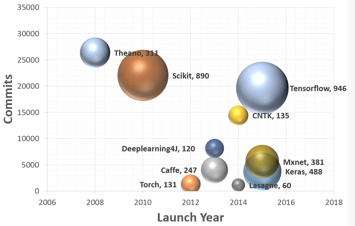
TensorFlow is a powerful open source software library developed by the Google Brain team for deep neural networks (DNNs). It was first made available under the Apache 2.x License in November 2015; as of today, its GitHub repository (https://github.com/tensorflow/tensorflow) has more than 17,000 commits, with roughly 845 contributors in just two years. This by itself is a measure of both the popularity and performance of TensorFlow. The following graph shows a comparison of the popular deep learning frameworks where it is clearly visible that TensorFlow is the leader among them:

Let's first learn what exactly TensorFlow is and why is it so popular among DNN researchers and engineers. TensorFlow, the open source deep learning library allows one to deploy deep neural networks computation on one or more CPU, GPUs in a server, desktop or mobile using the single TensorFlow API. You might ask, there are so many other deep learning libraries such as Torch, Theano, Caffe, and MxNet; what makes TensorFlow special? Most of other deep learning libraries like TensorFlow have auto-differentiation, many are open source, most support CPU/GPU options, have pretrained models, and support commonly used NN architectures like recurrent neural networks (RNNs), convolutional neural networks (CNNs), and deep belief networks (DBNs). So, what more is there in TensorFlow? Let's list them for you:

• It works with all the cool languages. TensorFlow works with Python, C++, Java, R, and Go.
• TensorFlow works on multiple platforms, even mobile and distributed.
• It is supported by all cloud providers--AWS, Google, and Azure.
• Keras, a high-level neural network API, has been integrated with TensorFlow.
• It has better computational graph visualizations because it is native while the equivalent in Torch/Theano is not nearly as cool to look at.
• TensorFlow allows model deployment and ease of use in production.
• TensorFlow has very good community support.
• TensorFlow is more than a software library; it is a suite of software that includes TensorFlow, TensorBoard, and TensorServing.

The Google research blog (https://research.googleblog.com/2016/11/celebrating-tensorflows-first-year.html) lists some of the fascinating projects done by people around the world using TensorFlow:

• Google Translate is using TensorFlow and tensor processing units (TPUs)
• Project Magenta, which can produce melodies using reinforcement learning-based models, employs TensorFlow
• Australian marine biologists are using TensorFlow to find and understand sea-cows, which are on the verge of extinction
• A Japanese farmer used TensorFlow to develop an application to sort cucumbers using physical parameters like size and shape

The list is long, and the possibilities in which one can use TensorFlow are even greater. This book aims to provide you with an understanding of TensorFlow as applied to deep learning models such that you can adapt them to your dataset with ease and develop useful applications. Each chapter contains a set of recipes which deal with the technical issues, the dependencies, the actual code, and its understanding. We have built the recipes one on another such that, by the end of each chapter, you have a fully functional deep learning model.

In this recipe, you will learn how to do a fresh installation of TensorFlow 1.3 on different OSes (Linux, Mac, and Windows). We will find out about the necessary requirements to install TensorFlow. TensorFlow can be installed using native pip, Anaconda, virtualenv, and Docker on Ubuntu and macOS. For Windows OS, one can use native pip or Anaconda.

As Anaconda works on all the three OSes and provides an easy way to not only install but also to maintain different project environments on the same system, we will concentrate on installing TensorFlow using Anaconda in this book. More details about Anaconda and managing its environment can be read from https://conda.io/docs/user-guide/index.html.

The code in this book has been tested on the following platforms:

• Windows 10, Anaconda 3, Python 3.5, TensorFlow GPU, CUDA toolkit 8.0, cuDNN v5.1, NVDIA® GTX 1070
• Windows 10/ Ubuntu 14.04/ Ubuntu 16.04/macOS Sierra, Anaconda3, Python 3.5, TensorFlow (CPU)

The prerequisite for TensorFlow installation is that the system has Python 2.5 or higher installed. The recipes in this book have been designed for Python 3.5 (the Anaconda 3 distribution). To get ready for the installation of TensorFlow, first ensure that you have Anaconda installed. You can download and install Anaconda for Windows/macOS or Linux from https://www.continuum.io/downloads.

After installation, you can verify the installation using the following command in your terminal window:

conda --version

Once Anaconda is installed, we move to the next step, deciding whether to install TensorFlow CPU or GPU. While almost all computer machines support TensorFlow CPU, TensorFlow GPU can be installed only if the machine has an NVDIA® GPU card with CUDA compute capability 3.0 or higher (minimum NVDIA® GTX 650 for desktop PCs).

For TensorFlow GPU, it is imperative that CUDA toolkit 7.0 or greater is installed, proper NVDIA® drivers are installed, and cuDNN v3 or greater is installed. On Windows, additionally, certain DLL files are needed; one can either download the required DLL files or install Visual Studio C++. One more thing to remember is that cuDNN files are installed in a different directory. One needs to ensure that directory is in the system path. One can also alternatively copy the relevant files in CUDA library in the respective folders.

We proceed with the recipe as follows:

1. Create a conda environment using the following at command line (If you are using Windows it will be better to do it as Administrator in the command line):

conda create -n tensorflow python=3.5

2. Activate the conda environment:

# Windows    
activate tensorflow
#Mac OS/ Ubuntu:    
source activate tensorflow
  

3. The command should change the prompt:

# Windows
(tensorflow)C:>
# Mac OS/Ubuntu    
(tensorflow)$

4. Next, depending on the TensorFlow version you want to install inside your conda environment, enter the following command:

## Windows
# CPU Version only
(tensorflow)C:>pip install --ignore-installed --upgrade https://storage.googleapis.com/tensorflow/windows/cpu/tensorflow-1.3.0cr2-cp35-cp35m-win_amd64.whl

# GPU Version  
(tensorflow)C:>pip install --ignore-installed --upgrade https://storage.googleapis.com/tensorflow/windows/gpu/tensorflow_gpu-1.3.0cr2-cp35-cp35m-win_amd64.whl

## Mac OS
# CPU only Version
(tensorflow)$ pip install --ignore-installed --upgrade https://storage.googleapis.com/tensorflow/mac/cpu/tensorflow-1.3.0cr2-py3-none-any.whl

# GPU version
(tensorflow)$ pip install --ignore-installed --upgrade https://storage.googleapis.com/tensorflow/mac/gpu/tensorflow_gpu-1.3.0cr2-py3-none-any.whl

## Ubuntu
# CPU only Version
(tensorflow)$ pip install --ignore-installed --upgrade https://storage.googleapis.com/tensorflow/linux/cpu/tensorflow-1.3.0cr2-cp35-cp35m-linux_x86_64.whl

# GPU Version
(tensorflow)$ pip install --ignore-installed --upgrade https://storage.googleapis.com/tensorflow/linux/gpu/tensorflow_gpu-1.3.0cr2-cp35-cp35m-linux_x86_64.whl

5. On the command line, type python.
6. Write the following code:

import tensorflow as tf
message = tf.constant('Welcome to the exciting world of Deep Neural Networks!')
with tf.Session() as sess:
    print(sess.run(message).decode())

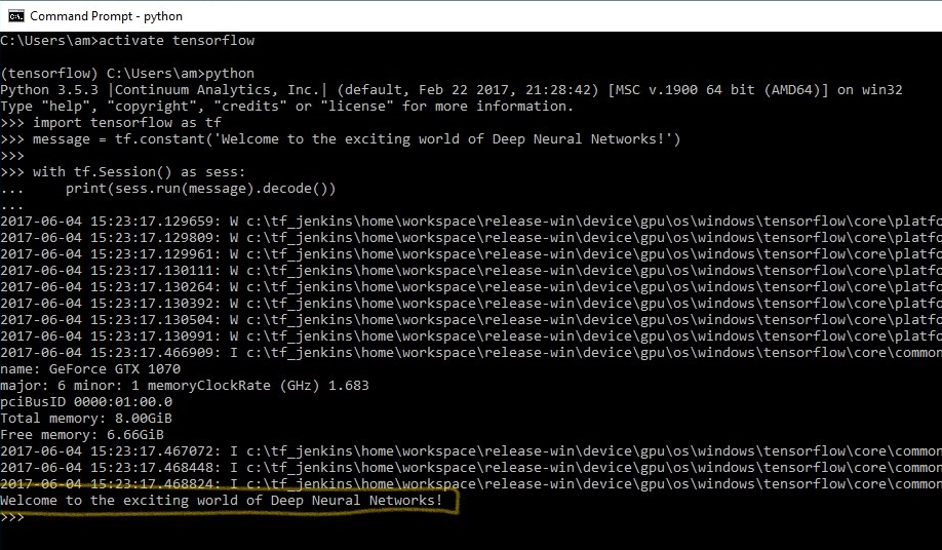
7. You will receive the following output:

8. Deactivate the conda environment at the command line using the command deactivate on Windows and source deactivate on MAC/Ubuntu.

TensorFlow is distributed by Google using the wheels standard. It is a ZIP format archive with the .whl extension. Python 3.6, the default Python interpreter in Anaconda 3, does not have wheels installed. At the time of writing the book, wheel support for Python 3.6 exists only for Linux/Ubuntu. Therefore, while creating the TensorFlow environment, we specify Python 3.5. This installs pip, python, and wheel along with a few other packages in the conda environment named tensorflow.

Once the conda environment is created, the environment is activated using the source activate/activate command. In the activated environment, use the pip install command with appropriate TensorFlow-API URL to install the required TensorFlow. Although there exists an Anaconda command to install TensorFlow CPU using conda forge TensorFlow documentation recommends using pip install. After installing TensorFlow in the conda environment, we can deactivate it. Now you are ready to execute your first TensorFlow program.

When the program runs, you may see a few warning (W) messages, some information (I) messages, and lastly the output of your code:

Welcome to the exciting world of Deep Neural Networks!

Congratulations for successfully installing and executing your first TensorFlow code! We will go through the code in more depth in the next recipe.

Additionally, you can also install Jupyter notebook:

1. Install ipython as follows:

conda install -c anaconda ipython
  

2. Install nb_conda_kernels:

conda install -channel=conda-forge nb_conda_kernels
  

3. Launch the Jupyter notebook:

jupyter notebook 

If you already have TensorFlow installed on your system, you can use pip install --upgrade tensorflow to upgrade it.

The first program that you learn to write in any computer language is Hello world. We maintain the convention in this book and start with the Hello world program. The code that we used in the preceding section to validate our TensorFlow installation is as follows:

import tensorflow as tf
message = tf.constant('Welcome to the exciting world of Deep Neural Networks!')
 with tf.Session() as sess:
     print(sess.run(message).decode()) 

Let's go in depth into this simple code.

1. Import tensorflow this imports the TensorFlow library and allows you to use its wonderful features.

 import tensorflow as tf 

2. Since the message we want to print is a constant string, we use tf.constant:

message = tf.constant('Welcome to the exciting world of Deep Neural Networks!')

3. To execute the graph element, we need to define the Session using with and run the session using run:

with tf.Session() as sess:
     print(sess.run(message).decode()) 

4. The output contains a series of warning messages (W), depending on your computer system and OS, claiming that code could run faster if compiled for your specific machine:

The TensorFlow library wasn't compiled to use SSE instructions, but these are available on your machine and could speed up CPU computations. 
The TensorFlow library wasn't compiled to use SSE2 instructions, but these are available on your machine and could speed up CPU computations. 
The TensorFlow library wasn't compiled to use SSE3 instructions, but these are available on your machine and could speed up CPU computations. 
The TensorFlow library wasn't compiled to use SSE4.1 instructions, but these are available on your machine and could speed up CPU computations. 
The TensorFlow library wasn't compiled to use SSE4.2 instructions, but these are available on your machine and could speed up CPU computations. 
The TensorFlow library wasn't compiled to use AVX instructions, but these are available on your machine and could speed up CPU computations. 
The TensorFlow library wasn't compiled to use AVX2 instructions, but these are available on your machine and could speed up CPU computations. 
The TensorFlow library wasn't compiled to use FMA instructions, but these are available on your machine and could speed up CPU computations. 

5. If you are working with TensorFlow GPU, you also get a list of informative messages (I) giving details of the devices used:

Found device 0 with properties:  
name: GeForce GTX 1070 
major: 6 minor: 1 memoryClockRate (GHz) 1.683 
pciBusID 0000:01:00.0 
Total memory: 8.00GiB 
Free memory: 6.66GiB 
DMA: 0  
0:   Y  
Creating TensorFlow device (/gpu:0) -> (device: 0, name: GeForce GTX 1070, pci bus id: 0000:01:00.0) 

6. At the end is the message we asked to print in the session:

Welcome to the exciting world of Deep Neural Networks

The preceding code is divided into three main parts. There is the import block that contains all the libraries our code will use; in the present code, we use only TensorFlow. The import tensorflow as tf statement gives Python access to all TensorFlow's classes, methods, and symbols. The second block contains the graph definition part; here, we build our desired computational graph. In the present case, our graph consists of only one node, the tensor constant message consisting of byte string, "Welcome to the exciting world of Deep Neural Networks". The third component of our code is running the computational graph as Session; we created a Session using the with keyword. Finally , in the Session, we run the graph created above.

Let's now understand the output. The warning messages that are received tell you that TensorFlow code could run at an even higher speed, which can be achieved by installing TensorFlow from source (we will do this in a later recipe in this chapter). The information messages received inform you about the devices used for computation. On their part, both messages are quite harmless, but if you don't like seeing them, adding this two-line code will do the trick:

import os
os.environ['TF_CPP_MIN_LOG_LEVEL']='2'   

The code is to ignore all messages till level 2. Level 1 is for information, 2 for warnings, and 3 for error messages.

The program prints the result of running the graph created the graph is run using the sess.run() statement. The result of running the graph is fed to the print function, which is further modified using the decode method. The sess.run evaluates the tensor defined in the message. The print function prints on stdout the result of the evaluation:

b'Welcome to the exciting world of Deep Neural Networks' 

This says that the result is a byte string. To remove string quotes and b (for byte), we use the method decode().

TensorFlow is very unlike other programming languages. We first need to build a blueprint of whatever neural network we want to create. This is accomplished by dividing the program into two separate parts, namely, definition of the computational graph and its execution. At first, this might appear cumbersome to the conventional programmer, but it is this separation of the execution graph from the graph definition that gives TensorFlow its strength, that is, the ability to work on multiple platforms and parallel execution.

Computational graph: A computational graph is a network of nodes and edges. In this section, all the data to be used, in other words, tensor Objects (constants, variables, and placeholders) and all the computations to be performed, namely, Operation Objects (in short referred as ops), are defined. Each node can have zero or more inputs but only one output. Nodes in the network represent Objects (tensors and Operations), and edges represent the Tensors that flow between operations. The computation graph defines the blueprint of the neural network but Tensors in it have no value associated with them yet.

To build a computation graph we define all the constants, variables, and operations that we need to perform. Constants, variables, and placeholders will be dealt with in the next recipe. Mathematical operations will be dealt in detail in the recipe for matrix manipulations. Here, we describe the structure using a simple example of defining and executing a graph to add two vectors.

Execution of the graph: The execution of the graph is performed using Session Object. The Session Object encapsulates the environment in which tensor and Operation Objects are evaluated. This is the place where actual calculations and transfer of information from one layer to another takes place. The values of different tensor Objects are initialized, accessed, and saved in Session Object only. Up to now the tensor Objects were just abstract definitions, here they come to life.

We proceed with the recipe as follows:

1. We consider a simple example of adding two vectors, we have two inputs vectors v_1 and v_2 they are to be fed as input to the Add operation. The graph we want to build is as follows:

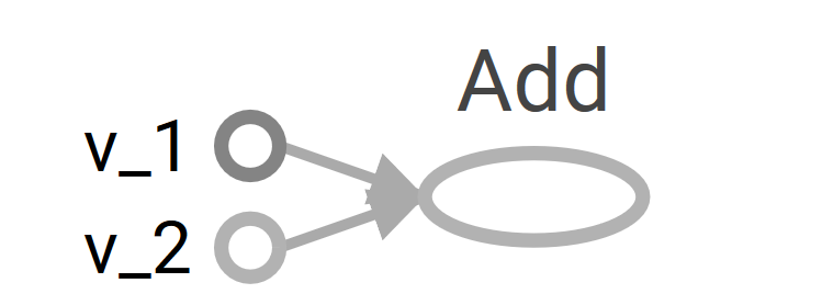
2. The corresponding code to define the computation graph is as follows:

v_1 = tf.constant([1,2,3,4]) 
v_2 = tf.constant([2,1,5,3]) 
v_add = tf.add(v_1,v_2)  # You can also write v_1 + v_2 instead 

3. Next, we execute the graph in the session:

with tf.Session() as sess: 
    prin(sess.run(v_add)) 

The above two commands are equivalent to the following code. The advantage of using with block is that one need not close the session explicitly.

sess = tf.Session() 
print(ses.run(tv_add)) 
sess.close() 

4. This results in printing the sum of two vectors:

[3 3 8 7] 

The building of a computational graph is very simple; you go on adding the variables and operations and passing them through (flow the tensors) in the sequence you build your neural network layer by layer. TensorFlow also allows you to use specific devices (CPU/GPU) with different objects of the computation graph using with tf.device(). In our example, the computational graph consists of three nodes, v_1 and v_2 representing the two vectors, and Add is the operation to be performed on them.

Now, to bring this graph to life, we first need to define a session object using tf.Session(); we gave the name sess to our session object. Next, we run it using the run method defined in Session class as follows:

run (fetches, feed_dict=None, options=None, run_metadata) 

This evaluates the tensor in fetches; our example has tensor v_add in fetches. The run method will execute every tensor and every operation in the graph leading to v_add. If instead of v_add, you have v_1 in fetches, the result will be the value of vector v_1:

[1,2,3,4]  

Fetches can be a single tensor/operation object or more, for example, if the fetches is [v_1, v_2, v_add], the output will be the following:

[array([1, 2, 3, 4]), array([2, 1, 5, 3]), array([3, 3, 8, 7])] 

In the same program code, we can have many session objects.

You must be wondering why we have to write so many lines of code for a simple vector addition or to print a small message. Well, you could have very conveniently done this work in a one-liner:

print(tf.Session().run(tf.add(tf.constant([1,2,3,4]),tf.constant([2,1,5,3])))) 

Writing this type of code not only affects the computational graph but can be memory expensive when the same operation ( OP) is performed repeatedly in a for loop. Making a habit of explicitly defining all tensor and operation objects not only makes the code more readable but also helps you visualize the computational graph in a cleaner manner.

If you are working on Jupyter Notebook or Python shell, it is more convenient to use tf.InteractiveSession instead of tf.Session. InteractiveSession makes itself the default session so that you can directly call run the tensor Object using eval() without explicitly calling the session, as described in the following example code:

sess = tf.InteractiveSession() 
 
v_1 = tf.constant([1,2,3,4]) 
v_2 = tf.constant([2,1,5,3]) 
 
v_add = tf.add(v_1,v_2) 
 
print(v_add.eval()) 
 
sess.close() 

TensorFlow in the simplest terms provides a library to define and perform different mathematical operations with tensors. A tensor is basically an n-dimensional matrix. All types of data, that is, scalar, vectors, and matrices are special types of tensors:

TensorFlow supports three types of tensors:

• Constants
• Variables
• Placeholders

Constants: Constants are the tensors whose values cannot be changed.

Variables: We use variable tensors when the values require updating within a session. For example, in the case of neural networks, the weights need to be updated during the training session, which is achieved by declaring weights as variables. The variables need to be explicitly initialized before use. Another important thing to note is that constants are stored in the computation graph definition; they are loaded every time the graph is loaded. In other words, they are memory expensive. Variables, on the other hand, are stored separately; they can exist on the parameter server.

Placeholders: These are used to feed values into a TensorFlow graph. They are used along with feed_dict to feed the data. They are normally used to feed new training examples while training a neural network. We assign a value to a placeholder while running the graph in the session. They allow us to create our operations and build the computation graph without requiring the data. An important point to note is that placeholders do not contain any data and thus there is no need to initialize them as well.

Let's start with constants:

1. We can declare a scalar constant:

t_1 = tf.constant(4)   

2. A constant vector of shape [1,3] can be declared as follows:

t_2 = tf.constant([4, 3, 2]) 

3. To create a tensor with all elements zero, we use tf.zeros(). This statement creates a zero matrix of shape [M,N] with dtype (int32, float32, and so on):

tf.zeros([M,N],tf.dtype)   

Let's take an example:

zero_t = tf.zeros([2,3],tf.int32) 
# Results in an 2×3 array of zeros: [[0 0 0], [0 0 0]] 

4. We can also create tensor constants of the same shape as an existing Numpy array or tensor constant as follows:

tf.zeros_like(t_2) 
# Create a zero matrix of same shape as t_2  
tf.ones_like(t_2) 
# Creates a ones matrix of same shape as t_2

5. We can create a tensor with all elements set to one; here, we create a ones matrix of shape [M,N]:

tf.ones([M,N],tf.dtype) 

Let's take an example:

ones_t = tf.ones([2,3],tf.int32) 
# Results in an 2×3 array of ones:[[1 1 1], [1 1 1]] 

Let's proceed to sequences:

1. We can generate a sequence of evenly spaced vectors, starting from start to stop, within total num values:

tf.linspace(start, stop, num) 

2. The corresponding values differ by (stop-start)/(num-1).
3. Let's take an example:

range_t = tf.linspace(2.0,5.0,5) 
# We get: [ 2.    2.75  3.5   4.25  5.  ]  

4. Generate a sequence of numbers starting from the start (default=0), incremented by delta (default =1), until, but not including, the limit:

tf.range(start,limit,delta) 

Here is an example:

range_t = tf.range(10) 
# Result: [0 1 2 3 4 5 6 7 8 9] 
 

TensorFlow allows random tensors with different distributions to be created:

1. To create random values from a normal distribution of shape [M,N] with the mean (default =0.0) and standard deviation (default=1.0) with seed, we can use the following:

t_random = tf.random_normal([2,3], mean=2.0, stddev=4, seed=12) 

# Result: [[ 0.25347459  5.37990952  1.95276058], [-1.53760314  1.2588985   2.84780669]]

2. To create random values from a truncated normal distribution of shape [M,N] with the mean (default =0.0) and standard deviation (default=1.0) with seed, we can use the following:

t_random = tf.truncated_normal([1,5], stddev=2, seed=12) 
# Result: [[-0.8732627 1.68995488 -0.02361972 -1.76880157 -3.87749004]]

3. To create random values from a given gamma distribution of shape [M,N] in the range [minval (default=0), maxval] with seed, perform as follows:

t_random = tf.random_uniform([2,3], maxval=4, seed=12) 

# Result: [[ 2.54461002  3.69636583  2.70510912], [ 2.00850058  3.84459829  3.54268885]] 

4. To randomly crop a given tensor to a specified size, do as follows:

tf.random_crop(t_random, [2,5],seed=12) 

Here, t_random is an already defined tensor. This will result in a [2,5] tensor randomly cropped from tensor t_random.

Many times we need to present the training sample in random order; we can use tf.random_shuffle() to randomly shuffle a tensor along its first dimension. If t_random is the tensor we want to shuffle, then we use the following:

tf.random_shuffle(t_random) 

5. Randomly generated tensors are affected by the value of the initial seed. To obtain the same random numbers in multiple runs or sessions, the seed should be set to a constant value. When there are large numbers of random tensors in use, we can set the seed for all randomly generated tensors using tf.set_random_seed(); the following command sets the seed for random tensors for all sessions as 54:

tf.set_random_seed(54)  

Let's now turn to the variables:

1. They are created using the variable class. The definition of variables also includes the constant/random values from which they should be initialized. In the following code, we create two different tensor variables, t_a and t_b. Both will be initialized to random uniform distributions of shape [50, 50], minval=0, and maxval=10:

rand_t = tf.random_uniform([50,50], 0, 10, seed=0) 
t_a = tf.Variable(rand_t) 
t_b = tf.Variable(rand_t) 

2. In the following code, we define two variables weights and bias. The weights variable is randomly initialized using normal distribution, with mean zeros and standard deviation of two, the size of weights is 100×100. The bias consists of 100 elements each initialized to zero. Here we have also used the optional argument name to give a name to the variable defined in the computational graph.

weights = tf.Variable(tf.random_normal([100,100],stddev=2)) 
bias = tf.Variable(tf.zeros[100], name = 'biases') 

3. In all the preceding examples, the source of initialization of variables is some constant. We can also specify a variable to be initialized from another variable; the following statement will initialize weight2 from the weights defined earlier:

weight2=tf.Variable(weights.initialized_value(), name='w2') 

4. The definition of variables specify how the variable is to be initialized, but we must explicitly initialize all declared variables. In the definition of the computational graph, we do it by declaring an initialization Operation Object:

intial_op = tf.global_variables_initializer(). 

5. Each variable can also be initialized separately using tf.Variable.initializer during the running graph:

bias = tf.Variable(tf.zeros([100,100]))
 with tf.Session() as sess:
     sess.run(bias.initializer)

6. Saving variables: We can save the variables using the Saver class. To do this, we define a saver Operation Object:

saver = tf.train.Saver()  

7. After constants and variables, we come to the most important element placeholders, they are used to feed data to the graph. We can define a placeholder using the following:

tf.placeholder(dtype, shape=None, name=None) 

8. dtype specifies the data type of the placeholder and must be specified while declaring the placeholder. Here, we define a placeholder for x and calculate y = 2 * x using feed_dict for a random 4×5 matrix:

x = tf.placeholder("float")
y = 2 * x
data = tf.random_uniform([4,5],10)
with tf.Session() as sess:
     x_data = sess.run(data)
     print(sess.run(y, feed_dict = {x:x_data})) 
 

To find out the value, we need to create the session graph and explicitly use the run command with the desired tensor values as fetches:

print(sess.run(t_1))  
# Will print the value of t_1 defined in step 1 

Very often, we will need constant tensor objects with a large size; in this case, to optimize memory, it is better to declare them as variables with a trainable flag set to False:

t_large = tf.Variable(large_array, trainable = False) 

TensorFlow was designed to work impeccably with Numpy, hence all the TensorFlow data types are based on those of Numpy. Using tf.convert_to_tensor(), we can convert the given value to tensor type and use it with TensorFlow functions and operators. This function accepts Numpy arrays, Python Lists, and Python scalars and allows interoperability with tensor Objects.

The following table lists some of the common TensorFlow supported data types (taken from TensorFlow.org):

Note that unlike Python/Numpy sequences, TensorFlow sequences are not iterable. Try the following code:

for i in tf.range(10)  

You will get an error:

#TypeError("'Tensor' object is not iterable.")

Matrix operations, such as performing multiplication, addition, and subtraction, are important operations in the propagation of signals in any neural network. Often in the computation, we require random, zero, ones, or identity matrices.

This recipe will show you how to get different types of matrices and how to perform different matrix manipulation operations on them.

We proceed with the recipe as follows:

1. We start an interactive session so that the results can be evaluated easily:

import tensorflow as tf

#Start an Interactive Session
sess = tf.InteractiveSession()

#Define a 5x5 Identity matrix
I_matrix = tf.eye(5)
print(I_matrix.eval()) 
# This will print a 5x5 Identity matrix

#Define a Variable initialized to a 10x10 identity matrix
X = tf.Variable(tf.eye(10))
X.initializer.run()  # Initialize the Variable
print(X.eval()) 
# Evaluate the Variable and print the result

#Create a random 5x10 matrix
A = tf.Variable(tf.random_normal([5,10]))
A.initializer.run()

#Multiply two matrices
product = tf.matmul(A, X)
print(product.eval())

#create a random matrix of 1s and 0s, size 5x10
b = tf.Variable(tf.random_uniform([5,10], 0, 2, dtype= tf.int32))
b.initializer.run()
print(b.eval())
b_new = tf.cast(b, dtype=tf.float32)
#Cast to float32 data type

# Add the two matrices
t_sum = tf.add(product, b_new)
t_sub = product - b_new
print("A*X _b\n", t_sum.eval())
print("A*X - b\n", t_sub.eval()) 
 

2. Some other useful matrix manipulations, like element-wise multiplication, multiplication with a scalar, elementwise division, elementwise remainder of a division, can be performed as follows:

import tensorflow as tf

# Create two random matrices
a = tf.Variable(tf.random_normal([4,5], stddev=2))
b = tf.Variable(tf.random_normal([4,5], stddev=2))

#Element Wise Multiplication
A = a * b

#Multiplication with a scalar 2
B = tf.scalar_mul(2, A)

# Elementwise division, its result is
C = tf.div(a,b)

#Element Wise remainder of division
D = tf.mod(a,b)

init_op = tf.global_variables_initializer()
with tf.Session() as sess:
     sess.run(init_op)
     writer = tf.summary.FileWriter('graphs', sess.graph)
     a,b,A_R, B_R, C_R, D_R = sess.run([a , b, A, B, C, D])
     print("a\n",a,"\nb\n",b, "a*b\n", A_R, "\n2*a*b\n", B_R, "\na/b\n", C_R, "\na%b\n", D_R)

writer.close() 

All arithmetic operations of matrices like add, sub, div, multiply (elementwise multiplication), mod, and cross require that the two tensor matrices should be of the same data type. In case this is not so they will produce an error. We can use tf.cast() to convert Tensors from one data type to another.

If we are doing division between integer tensors, it is better to use tf.truediv(a,b) as it first casts the integer tensors to floating points and then performs element-wise division.

1. The first step in using TensorBoard is to identify which OPs summaries you would like to have. In the case of DNNs, it is customary to know how the loss term (objective function) varies with time. In the case of Adaptive learning rate, the learning rate itself varies with time. We can get the summary of the term we require with the help of tf.summary.scalar OPs. Suppose, the variable loss defines the error term and we want to know how it varies with time, then we can do this as follows:

loss = tf... 
tf.summary.scalar('loss', loss) 

2. You can also visualize the distribution of gradients, weights, or even output of a particular layer using tf.summary.histogram:

output_tensor  = tf.matmul(input_tensor, weights) + biases 
tf.summary.histogram('output', output_tensor)

3. The summaries will be generated during the session. Instead of executing every summary operation individually, you can define tf.merge_all_summaries OPs in the computation graph to get all summaries in a single run.
4. The generated summary then needs to be written in an event file using tf.summary.Filewriter:

writer = tf.summary.Filewriter('summary_dir', sess.graph) 

5. This writes all the summaries and the graph in the 'summary_dir' directory.
6. Now, to visualize the summaries, you need to invoke TensorBoard from the command line:

tensorboard --logdir=summary_dir 

7. Next, open your browser and type the address http://localhost:6006/ (or the link you received after running the TensorBoard command).
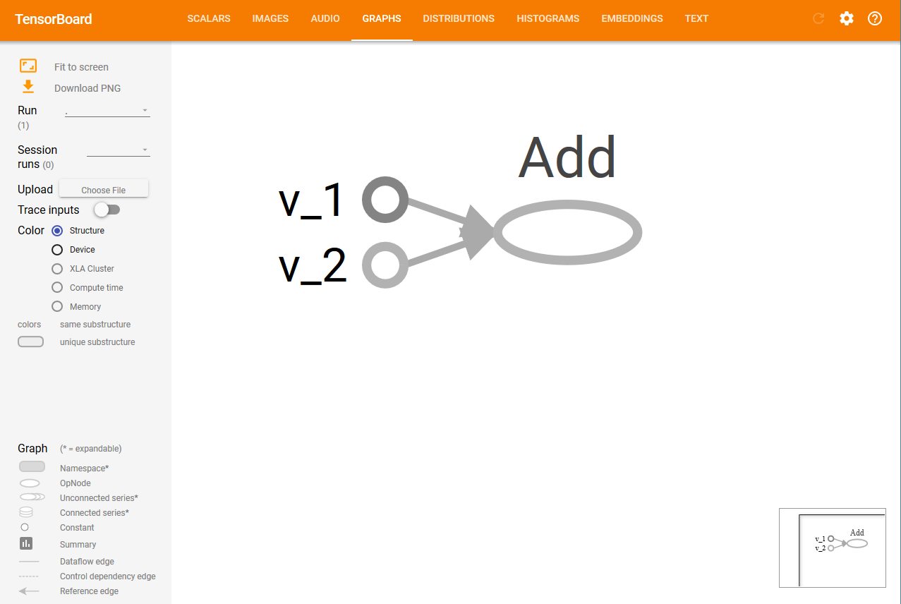
8. You will see something like the following, with many tabs on the top. The Graphs tab will display the graph:

TensorFlow 1.x does not offer backward compatibility. This means that the codes that worked on TensorFlow 0.x may not work on TensorFlow 1.0. So, if you have codes that worked on TensorFlow 0.x, you need to upgrade them (old GitHub repositories or your own codes). This recipe will point out major differences between TensorFlow 0.x and TensorFlow 1.0 and will show you how to use the script tf_upgrade.py to automatically upgrade the code for TensorFlow 1.0.

Here is how we proceed with the recipe:

1. First, download tf_upgrade.py from https://github.com/tensorflow/tensorflow/tree/master/tensorflow/tools/compatibility.
2. If you want to convert one file from TensorFlow 0.x to TensorFlow 1.0, use the following command at the command line:

python tf_upgrade.py --infile old_file.py --outfile upgraded_file.py
  

3. For example, if you have a TensorFlow program file named test.py, you will use the preceding command as follows:

python tf_upgrade.py --infile test.py --outfile test_1.0.py

4. This will result in the creation of a new file named test_1.0.py.
5. If you want to migrate all the files of a directory, then use the following at the command line:

python tf_upgrade.py --intree InputDIr --outtree OutputDir
 # For example, if you have a directory located at /home/user/my_dir you can migrate all the python files in the directory located at /home/user/my-dir_1p0 using the above command as:
python tf_upgrade.py --intree /home/user/my_dir --outtree /home/user/my_dir_1p0

6. In most cases, the directory also contains dataset files; you can ensure that non-Python files are copied as well in the new directory (my-dir_1p0 in the preceding example) using the following:

python tf_upgrade.py --intree /home/user/my_dir --outtree /home/user/my_dir_1p0 -copyotherfiles True
  

7. In all these cases, a report.txt file is generated. This file contains the details of conversion and any errors in the process.
8. Read the report.txt file and manually upgrade the part of the code that the script is unable to update.

tf_upgrade.py has certain limitations:

• It cannot change the arguments of tf.reverse(): you will have to manually fix it
• For methods with argument list reordered, like tf.split() and tf.reverse_split(), it will try to introduce keyword arguments, but it cannot actually reorder the arguments
• You will have to manually replace constructions like tf.get.variable_scope().reuse_variables() with the following:

with tf.variable_scope(tf.get_variable_scope(), resuse=True):

Accelerated linear algebra (XLA) is a domain-specific compiler for linear algebra. According to https://www.tensorflow.org/performance/xla/, it is still in the experimental stage and is used to optimize TensorFlow computations. It can provide improvements in execution speed, memory usage, and portability on the server and mobile platforms. It provides two-way JIT (Just In Time) compilation or AoT (Ahead of Time) compilation. Using XLA, you can produce platform-dependent binary files (for a large number of platforms like x64, ARM, and so on), which can be optimized for both memory and speed.

At present, XLA is not included in the binary distributions of TensorFlow. One needs to build it from source. To build TensorFlow from source, knowledge of LLVM and Bazel along with TensorFlow is required. TensorFlow.org supports building from source in only MacOS and Ubuntu. The steps needed to build TensorFlow from the source are as follows (https://www.tensorflow.org/install/install_sources):

1. Determine which TensorFlow you want to install--TensorFlow with CPU support only or TensorFlow with GPU support.
2. Clone the TensorFlow repository:

git clone https://github.com/tensorflow/tensorflow 
cd tensorflow 
git checkout Branch #where Branch is the desired branch  

3. Install the following dependencies:

• • Bazel
  • TensorFlow Python dependencies
  • For the GPU version, NVIDIA packages to support TensorFlow

4. Configure the installation. In this step, you need to choose different options such as XLA, Cuda support, Verbs, and so on:

./configure 

5. Next, use bazel-build:
6. For CPU only version you use:

bazel build --config=opt //tensorflow/tools/pip_package:build_pip_package
      

7. If you have a compatible GPU device and you want the GPU Support, then use:

bazel build --config=opt --config=cuda //tensorflow/tools/pip_package:build_pip_package
  

8. On a successful run, you will get a script, build_pip_package.
9. Run this script as follows to build the whl file:

bazel-bin/tensorflow/tools/pip_package/build_pip_package /tmp/tensorflow_pkg

10. Install the pip package:

sudo pip install /tmp/tensorflow_pkg/tensorflow-1.1.0-py2-none-any.whl
  

Now you are ready to go.

TensorFlow generates TensorFlow graphs. With the help of XLA, it is possible to run the TensorFlow graphs on any new kind of device.

1. JIT Compilation: This is to turn on JIT compilation at session level:

# Config to turn on JIT compilation
 config = tf.ConfigProto()
 config.graph_options.optimizer_options.global_jit_level = tf.OptimizerOptions.ON_1

 sess = tf.Session(config=config) 

2. This is to turn on JIT compilation manually:

jit_scope = tf.contrib.compiler.jit.experimental_jit_scope

x = tf.placeholder(np.float32)
with jit_scope():
   y = tf.add(x, x)  # The "add" will be compiled with XLA. 

3. We can also run computations via XLA by placing the operator on a specific XLA device XLA_CPU or XLA_GPU:

with tf.device \ ("/job:localhost/replica:0/task:0/device:XLA_GPU:0"):
   output = tf.add(input1, input2) 

AoT Compilation: Here, we use tfcompile as standalone to convert TensorFlow graphs into executable code for different devices (mobile).

TensorFlow.org tells about tfcompile:

For advanced steps to do the same, you can refer to https://www.tensorflow.org/performance/xla/tfcompile.

TensorFlow supports both CPUs and GPUs. It also supports distributed computation. We can use TensorFlow on multiple devices in one or more computer system. TensorFlow names the supported devices as "/device:CPU:0" (or "/cpu:0") for the CPU devices and "/device:GPU:I" (or "/gpu:I") for the i^th GPU device.

As mentioned earlier, GPUs are much faster than CPUs because they have many small cores. However, it is not always an advantage in terms of computational speed to use GPUs for all types of computations. The overhead associated with GPUs can sometimes be more computationally expensive than the advantage of parallel computation offered by GPUs. To deal with this issue, TensorFlow has provisions to place computations on a particular device. By default, if both CPU and GPU are present, TensorFlow gives priority to GPU.

TensorFlow represents devices as strings. Here, we will show you how one can manually assign a device for matrix multiplication in TensorFlow. To verify that TensorFlow is indeed using the device (CPU or GPU) specified, we create the session with the log_device_placement flag set to True, namely, config=tf.ConfigProto(log_device_placement=True):

1. If you are not sure about the device and want TensorFlow to choose the existing and supported device, you can set the allow_soft_placement flag to True:

config=tf.ConfigProto(allow_soft_placement=True, log_device_placement=True) 

2. Manually select CPU for operation:

with tf.device('/cpu:0'): 
    rand_t = tf.random_uniform([50,50], 0, 10, dtype=tf.float32, seed=0) 
    a = tf.Variable(rand_t) 
    b = tf.Variable(rand_t) 
    c = tf.matmul(a,b) 
    init = tf.global_variables_initializer() 
 
sess = tf.Session(config) 
sess.run(init) 
print(sess.run(c))    

3. We get the following output:

We can see that all the devices, in this case, are '/cpu:0'.

4. Manually select a single GPU for operation:

with tf.device('/gpu:0'): 
    rand_t = tf.random_uniform([50,50], 0, 10, dtype=tf.float32, seed=0) 
    a = tf.Variable(rand_t) 
    b = tf.Variable(rand_t) 
    c = tf.matmul(a,b) 
    init = tf.global_variables_initializer() 
 
sess = tf.Session(config=tf.ConfigProto(log_device_placement=True)) 
sess.run(init) 
print(sess.run(c)) 

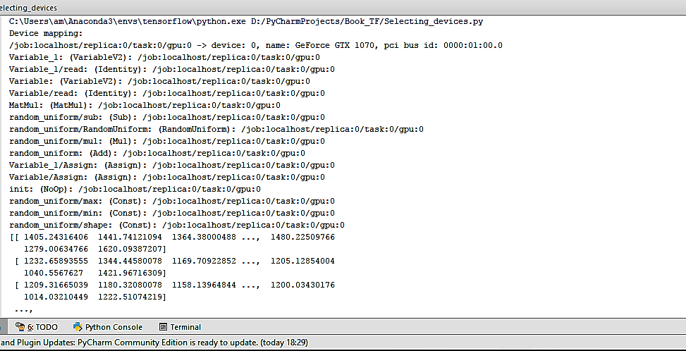
5. The output now changes to the following:

6. The '/cpu:0' after each operation is now replaced by '/gpu:0'.
7. Manually select multiple GPUs:

c=[]
for d in ['/gpu:1','/gpu:2']:
     with tf.device(d):
         rand_t = tf.random_uniform([50, 50], 0, 10, dtype=tf.float32, seed=0)
         a = tf.Variable(rand_t)
         b = tf.Variable(rand_t)
         c.append(tf.matmul(a,b))
         init = tf.global_variables_initializer()

sess = tf.Session(config=tf.ConfigProto(allow_soft_placement=True,log_device_placement=True))
sess.run(init)
print(sess.run(c))
sess.close() 

8. In this case, if the system has three GPU devices, then the first set of multiplication will be carried on by '/gpu:1' and the second set by '/gpu:2'.

The tf.device() argument selects the device (CPU or GPU). The with block ensures the operations for which the device is selected. All the variables, constants, and operations defined within the with block will use the device selected in tf.device(). Session configuration is controlled using tf.ConfigProto. By setting the allow_soft_placement and log_device_placement flags, we tell TensorFlow to automatically choose the available devices in case the specified device is not available, and to give log messages as output describing the allocation of devices while the session is executed.

DNNs today is the buzzword in the AI community. Many data science/Kaggle competitions have been recently won by candidates using DNNs. While the concept of DNNs had been around since the proposal of Perceptrons by Rosenblat in 1962 and they were made feasible by the discovery of the Gradient Descent Algorithm in 1986 by Rumelhart, Hinton, and Williams. It is only recently that DNNs became the favourite of AI/ML enthusiasts and engineers world over.

The main reason for this is the availability of modern computing power such as GPUs and tools like TensorFlow that make it easier to access GPUs and construct complex neural networks in just a few lines of code.

As a machine learning enthusiast, you must already be familiar with the concepts of neural networks and deep learning, but for the sake of completeness, we will introduce the basics here and explore what features of TensorFlow make it a popular choice for deep learning.

Neural networks are a biologically inspired model for computation and learning. Like a biological neuron, they take weighted input from other cells (neurons or environment); this weighted input undergoes a processing element and results in an output which can be binary (fire or not fire) or continuous (probability, prediction). Artificial Neural Networks (ANNs) are networks of these neurons, which can be randomly distributed or arranged in a layered structure. These neurons learn through the set of weights and biases associated with them.

The following figure gives a good idea about the similarity of the neural network in biology and an artificial neural network:

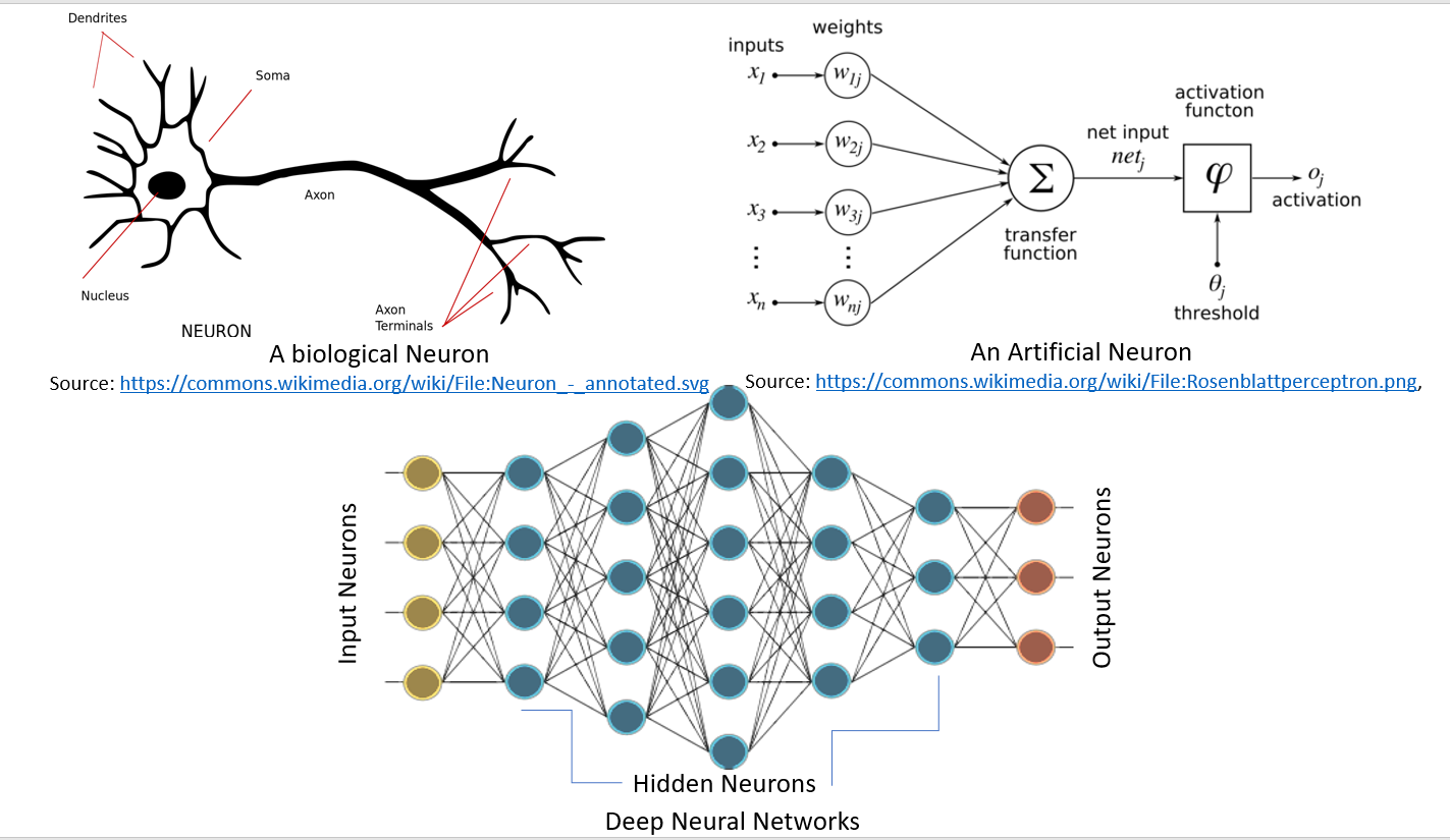
Deep learning, as defined by Hinton et al. (https://www.cs.toronto.edu/~hinton/absps/NatureDeepReview.pdf), consists of computational models composed of multiple processing layers (hidden layers). An increase in the number of layers results in an increase in learning time. The learning time further increases due to a large dataset, as is the norm of present-day CNN or Generative Adversarial Networks (GANs). Thus, to practically implement DNNs, we require high computation power. The advent of GPUs by NVDIA® made it feasible and then TensorFlow by Google made it possible to implement complex DNN structures without going into the complex mathematical details, and availability of large datasets provided the necessary food for DNNs. TensorFlow is the most popular library for deep learning for the following reasons:

• TensorFlow is a powerful library for performing large-scale numerical computations like matrix multiplication or auto-differentiation. These two computations are necessary to implement and train DNNs.
• TensorFlow uses C/C++ at the backend, which makes it computationally fast.
• TensorFlow has a high-level machine learning API (tf.contrib.learn) that makes it easier to configure, train, and evaluate a large number of machine learning models.
• One can use Keras, a high-level deep learning library, on top of TensorFlow. Keras is very user-friendly and allows easy and fast prototyping. It supports various DNNs like RNNs, CNNs, and even a combination of the two.

Any deep learning network consists of four important components: Dataset, defining the model (network structure), Training/Learning, and Prediction/Evaluation. We can do all these in TensorFlow; let's see how:

• Dataset: DNNs depend on large amounts of data. The data can be collected or generated or one can also use standard datasets available. TensorFlow supports three main methods to read the data. There are different datasets available; some of the datasets we will be using to train the models built in this book are as follows:
• MNIST: It is the largest database of handwritten digits (0 - 9). It consists of a training set of 60,000 examples and a test set of 10,000 examples. The dataset is maintained at Yann LeCun's home page (http://yann.lecun.com/exdb/mnist/). The dataset is included in the TensorFlow library in tensorflow.examples.tutorials.mnist.
• CIFAR10: This dataset contains 60,000 32 x 32 color images in 10 classes, with 6,000 images per class. The training set contains 50,000 images and test dataset--10,000 images. The ten classes of the dataset are: airplane, automobile, bird, cat, deer, dog, frog, horse, ship, and truck. The data is maintained by the Computer Science Department, University of Toronto (https://www.cs.toronto.edu/~kriz/cifar.html).
• WORDNET: This is a lexical database of English. It contains nouns, verbs, adverbs, and adjectives, grouped into sets of cognitive synonyms (Synsets), that is, words that represent the same concept, for example, shut and close or car and automobile are grouped into unordered sets. It contains 155,287 words organised in 117,659 synsets for a total of 206,941 word-sense pairs. The data is maintained by Princeton University (https://wordnet.princeton.edu/).

• ImageNET: This is an image dataset organized according to the WORDNET hierarchy (only nouns at present). Each meaningful concept (synset) is described by multiple words or word phrases. Each synset is represented on average by 1,000 images. At present, it has 21,841 synsets and a total of 14,197,122 images. Since 2010, an annual ImageNet Large Scale Visual Recognition Challenge (ILSVRC) has been organized to classify images in one of the 1,000 object categories. The work is sponsored by Princeton University, Stanford University, A9, and Google (http://www.image-net.org/).
• YouTube-8M: This is a large-scale labelled video dataset consisting of millions of YouTube videos. It has about 7 million YouTube video URLs classified into 4,716 classes, organized into 24 top-level categories. It also provides preprocessing support and frame-level features. The dataset is maintained by Google Research (https://research.google.com/youtube8m/).

Reading the data: The data can be read in three ways in TensorFlow--feeding through feed_dict, reading from files, and using preloaded data. We will be using the components described in this recipe throughout the book for reading, and feeding the data. In the next steps, you will learn each one of them.

1. Feeding: In this case, data is provided while running each step, using the feed_dict argument in the run() or eval() function call. This is done with the help of placeholders and this method allows us to pass Numpy arrays of data. Consider the following part of code using TensorFlow:

... 
y = tf.placeholder(tf.float32) 
x = tf.placeholder(tf.float32). 
... 
with tf.Session as sess: 
   X_Array = some Numpy Array 
   Y_Array = other Numpy Array 
   loss= ... 
sess.run(loss,feed_dict = {x: X_Array, y: Y_Array}). 
... 

Here, x and y are the placeholders; using them, we pass on the array containing X values and the array containing Y values with the help of feed_dict.

2. Reading from files: This method is used when the dataset is very large to ensure that not all data occupies the memory at once (imagine the 60 GB YouTube-8m dataset). The process of reading from files can be done in the following steps:

• • A list of filenames is created using either string Tensor ["file0", "file1"] or [("file%d"i) for in in range(2)] or using the files = tf.train.match_filenames_once('*.JPG') function.

• • Filename queue: A queue is created to keep the filenames until the reader needs them using the tf.train.string_input_producer function:

filename_queue = tf.train.string_input_producer(files) 
# where files is the list of filenames created above 

This function also provides an option to shuffle and set a maximum number of epochs. The whole list of filenames is added to the queue for each epoch. If the shuffling option is selected (shuffle=True), then filenames are shuffled in each epoch.

• • Reader is defined and used to read from files from the filename queue. The reader is selected based on the input file format. The read method a key identifying the file and record (useful while debugging) and a scalar string value. For example, in the case of .csv file formats:

reader = tf.TextLineReader() 
key, value = reader.read(filename_queue)

• • Decoder: One or more decoder and conversion ops are then used to decode the value string into Tensors that make up the training example:

record_defaults = [[1], [1], [1]]
col1, col2, col3 = tf.decode_csv(value, record_defaults=record_defaults) 
 

3. Preloaded data: This is used when the dataset is small and can be loaded fully in the memory. For this, we can store data either in a constant or variable. While using a variable, we need to set the trainable flag to False so that the data does not change while training. As TensorFlow constants:

# Preloaded data as constant
training_data = ... 
training_labels = ... 
with tf.Session as sess: 
   x_data = tf.Constant(training_data) 
   y_data = tf.Constant(training_labels) 
...

# Preloaded data as Variables
training_data = ... 
training_labels = ... 
with tf.Session as sess: 
   data_x = tf.placeholder(dtype=training_data.dtype, shape=training_data.shape) 
   data_y = tf.placeholder(dtype=training_label.dtype, shape=training_label.shape) 
   x_data = tf.Variable(data_x, trainable=False, collections[]) 
   y_data = tf.Variable(data_y, trainable=False, collections[]) 
... 

Conventionally, the data is divided into three parts--training data, validation data, and test data.

4. Defining the model: A computational graph is built describing the network structure. It involves specifying the hyperparameters, variables, and placeholders sequence in which information flows from one set of neurons to another and a loss/error function. You will learn more about the computational graphs in a later section of this chapter.

5. Training/Learning: The learning in DNNs is normally based on the gradient descent algorithm, (it will be dealt in detail in Chapter 2, Regression) where the aim is to find the training variables (weights/biases) such that the error or loss (as defined by the user in step 2) is minimized. This is achieved by initializing the variables and using run():

with tf.Session as sess: 
   .... 
   sess.run(...) 
   ... 

6. Evaluating the model: Once the network is trained, we evaluate the network using predict() on validation data and test data. The evaluations give us an estimate of how well our model fits the dataset. We can thus avoid the common mistakes of overfitting or underfitting. Once we are satisfied with our model, we can deploy it in production.

In TensorFlow 1.3, a new feature called TensorFlow Estimators has been added. TensorFlow Estimators make the task of creating the neural network models even easier, it is a higher level API that encapsulates the process of training, evaluation, prediction and serving. It provides the option of either using pre-made Estimators or one can write their own custom Estimators. With pre-made Estimators, one no longer have to worry about building the computational or creating a session, it handles it all.

At present TensorFlow Estimator has six pre-made Estimators. Another advantage of using TensorFlow pre-made Estimators is that it also by itself creates summaries that can be visualised on TensorBoard. More details about Estimators are available at https://www.tensorflow.org/programmers_guide/estimators.

TensorFlow takes care of most of the neural network implementation. However, this is not sufficient; for preprocessing tasks, serialization, and even plotting, we need some more Python packages.

Here are listed some of the common Python packages used:

1. Numpy: This is the fundamental package for scientific computing with Python. It supports n-dimensional arrays and matrices. It also has a large collection of high-level mathematical functions. It is a necessary package required by TensorFlow and therefore, with pip install tensorflow, it is installed if not already present.
2. Matplolib: This is the Python 2D plotting library. You can use it to create plots, histograms, bar charts, error charts, scatterplots, and power spectra with just a few lines of code. It can be installed using pip:

pip install matplotlib 
# or using Anaconda    
conda install -c conda-forge matplotlib

3. OS: This is included in the basic Python installation. It provides an easy and portable way of using operating system-dependent functionality like reading, writing, and changing files and directories.
4. Pandas: This provides various data structures and data analysis tools. Using Pandas, you can read and write data between in-memory data structures and different formats. We can read from .csv and text files. It can be installed using either pip install or conda install.
5. Seaborn: This is a specialized statistical data visualization tool built on Matplotlib.
6. H5fs: H5fs is a filesystem for Linux (also other operating systems with FUSE implementation like macOS X) capable of operations on an HDFS (Hierarchical Data Format Filesystem).
7. PythonMagick: It is the Python binding of the ImageMagick library. It is a library to display, convert, and edit raster image and vector image files. It supports more than 200 image file formats. It can be installed using source build available from ImageMagick. Certain .whl formats are also available for a convenient pip install (http://www.lfd.uci.edu/%7Egohlke/pythonlibs/#pythonmagick).

8. TFlearn: TFlearn is a modular and transparent deep learning library built on top of TensorFlow. It provides a higher-level API to TensorFlow in order to facilitate and speed up experimentation. It currently supports most of the recent deep learning models, such as Convolutions, LSTM, BatchNorm, BiRNN, PReLU, Residual networks, and Generative networks. It works only for TensorFlow 1.0 or higher. To install, use pip install tflearn.
9. Keras: Keras too is a high-level API for neural networks, which uses TensorFlow as its backend. It can run on top of Theano and CNTK as well. It is extremely user-friendly, adding layers to it is just a one-line job. It can be installed using pip install keras.

Below you can find some weblinks for more information on installation of TensorFlow

• https://www.tensorflow.org/install/
• https://www.tensorflow.org/install/install_sources
• http://llvm.org/
• https://bazel.build/