


Data consists of observations across different types of variables, and it is vital that any data analyst understands these intricacies at the earliest stage of exposure to statistical analysis. This chapter recognizes the importance of data and begins with a template of a dummy questionnaire and then proceeds with the nitty-gritties of the subject. We will then explain how uncertainty creeps in to the domain of computer science. The chapter closes with coverage of important families of discrete and continuous random variables.
We will cover the following topics:
Identification of the main variable types as nominal, categorical, and continuous variables
The uncertainty arising in many real experiments
R installation and packages
The mathematical form of discrete and continuous random variables and their applications
The goal of this section is to introduce numerous variable types at the first possible occasion. Traditionally, an introductory course begins with the elements of probability theory and then builds up the requisites leading to random variables. This convention is dropped in this book and we begin straightaway with, data. There is a primary reason for choosing this path. The approach builds on what the reader is already familiar with and then connects it with the essential framework of the subject.
It is very likely that the user is familiar with questionnaires. A questionnaire may be asked after the birth of a baby with a view to aid the hospital in the study about the experience of the mother, the health status of the baby, and the concerns of the immediate guardians of the new born. A multi-store department may instantly request the customer to fill in a short questionnaire for capturing the customer’s satisfaction after the sale of a product. Customer’s satisfaction following the service of their vehicle (see the detailed example discussed later) can be captured through a few queries.
The questionnaires may arise in different forms than merely on a physical paper. They may be sent via email, telephone, short message service (SMS), and so on. As an example, one may receive an SMS that seeks a mandatory response in a Yes/No form. An email may arrive in an Outlook inbox, which requires the recipient to respond through a vote for any of these three options, Will attend the meeting, Can’t attend the meeting, or Not yet decided.
Suppose the owner of a multi-brand car center wants to find out the satisfaction percentage of his customers. Customers bring their car to a service center for varied reasons. The owner wants to find out the satisfaction levels post the servicing of the cars and find the areas where improvement will lead to higher satisfaction among the customers. It is well known that the higher the satisfaction levels, the greater would be the customer’s loyalty towards the service center. Towards this, a questionnaire is designed and then data is collected from the customers. A snippet of the questionnaire is given in the following figure, and the information given by the customers leads to different types of data characteristics.
The Customer ID and Questionnaire ID variables may be serial numbers, or randomly generated unique numbers. The purpose of such variables is unique identification of people’s responses. It may be possible that there are follow-up questionnaires as well. In such cases, the Customer ID for a responder will continue to be the same, whereas the Questionnaire ID needs to change for the identification of the follow up. The values of these types of variables in general are not useful for analytical purposes.
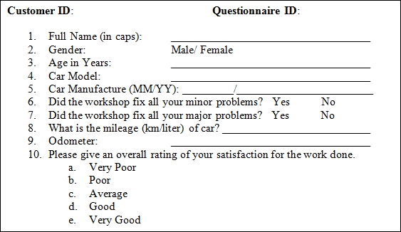
A hypothetical questionnaire
The information of FullName in this survey is a beginning point to break the ice with the responder. In very exceptional cases the name may be useful for profiling purposes. For our purposes the name will simply be a text variable that is not used for analysis purposes. Gender is asked to know the person’s gender and in quite a few cases it may be an important factor explaining the main characteristics of the survey; in this case it may be mileage. Gender is an example of a categorical variable.
Age in Years is a variable that captures the age of the customer. The data for this field is numeric in nature and is an example of a continuous variable.
The fourth and fifth questions help the multi-brand dealer in identifying the car model and its age. The first question here enquires about the type of the car model. The car models of the customers may vary from Volkswagen Beetle, Ford Endeavor, Toyota Corolla, Honda Civic, to Tata Nano (see the following screenshot). Though the model name is actually a noun, we make a distinction from the first question of the questionnaire in the sense that the former is a text variable while the latter leads to a categorical variable. Next, the car model may easily be identified to classify the car into one of the car categories, such as a hatchback, sedan, station wagon, or utility vehicle, and such a classifying variable may serve as one of the ordinal variable, as per the overall car size. The age of the car in months since its manufacture date may explain the mileage and odometer reading.
The sixth and seventh questions simply ask the customer if their minor/major problems were completely fixed or not. This is a binary question that takes either of the values, Yes or No. Small dents, power windows malfunctioning, a niggling noise in the cabin, music speakers low output, and other similar issues, which do not lead to good functioning of the car, may be treated as minor problems that are expected to be fixed in the car. Disc brake problems, wheel alignment, steering rattling issues, and similar problems that expose the user and co-users of the road to danger are of grave concerns as they affect the functioning of a car and are treated as major problems. Any user will expect all his issues to be resolved during a car service. An important goal of the survey is to find the service center efficiency in handling the minor and major issues of the car. The labels Yes/No may be replaced by a +1 and -1 combination, or any other label of convenience.
The eighth question, What is the mileage (km/liter) of car?, gives a measure of the average petrol/diesel consumption. In many practical cases, this data is provided by the belief of the customer who may simply declare it between 5 km/liter to 25 km/liter. In the case of a lower mileage, the customer may ask for a finer tune up of the engine, wheel alignment, and so on. A general belief is that if the mileage is closer to the assured mileage as marketed by the company, or some authority such as Automotive Research Association of India (ARAI), the customer is more likely to be happy. An important variable is the overall kilometers done by the car up to the point of service. Vehicles have certain maintenances at the intervals of 5,000 km, 10,000 km, 20,000 km, 50,000 km, and 100,000 km. This variable may also be related to the age of the vehicle.
Let us now look at the final question of the snippet. Here, the customer is asked to rate his overall experience of the car service. A response from the customer may be sought immediately after a small test ride post the car service, or it may be through a questionnaire sent to the customer’s email ID. A rating of Very Poor suggests that the workshop has served the customer miserably, whereas a rating of Very Good conveys that the customer is completely satisfied with the workshop service.
Note that there is some order in the response of the customer, in that we can grade the ranking in a certain order of Very Poor < Poor < Average < Good < Very Good. This implies that the structure of the ratings must be respected when we analyze the data of such a study. In the next section, these concepts are elaborated through a hypothetical dataset.
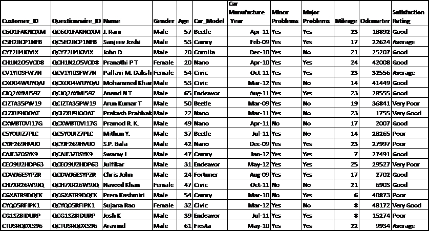
Hypothetical DataSet of a Questionnaire
A snippet of an R session is given in the following figure . Here we simply relate an R session with the survey and sample data of the previous table. The simple goal here is to get a feel/buy-in of R and not necessarily follow the R codes. The R installation process is explained in the R installation section. Here the user is loading the SQ R data object (SQ simply stands for sample questionnaire) in the session. The nature of the SQ object is a data.frame that stores a variety of other objects in itself. For more technical details of the data.frame function, see The data.frame object section of Chapter 2, Import/Export Data. The names of a data.frame object may be extracted using the variable.names function. The R function class helps to identify the nature of the R object. As we have a list of variables, it is useful to find all of them using the sapply function. In the following screenshot, the mentioned steps have been carried out:
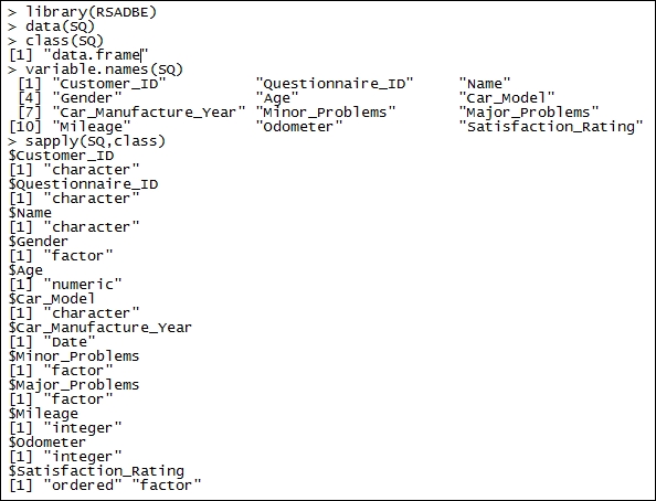
Understanding variable types of an R object
The variable characteristics are also on the expected lines, as they should be, and we see that the variables Customer_ID, Questionnaire_ID, and Name are character variables; Gender, Car_Model, Minor_Problems, and Major_Problems are factor variables; DoB and Car_Manufacture_Year are date variables; Mileage and Odometer are integer variables; and, finally, the variable Satisfaction_Rating is an ordered and factor variable.
In the remainder of the chapter, we will delve into more details about the nature of various data types. In a more formal language, a variable is called a random variable (RV) in the rest of the book, and in the statistical literature. A distinction needs to be made here. In this book, we do not focus on the important aspects of probability theory. It is assumed that the reader is familiar with probability, say at the level of Freund (2003) or Ross (2001). An RV is a function that is mapping from the probability (sample) space 
to the real line. From the previous example, we have Odometer and Satisfaction_Rating as two examples of a random variable. In a formal language, the random variables are generally denoted by letters X, Y, …. The distinction that is required here is that in the applications that we observe are the realizations/values of the random variables. In general, the realized values are denoted by the lower cases x, y, …. Let us clarify this at more length.
Suppose that we denote the random variable Satisfaction_Rating by X. Here, the sample space consists of the elements Very Poor, Poor, Average, Good, and Very Good. For the sake of convenience, we will denote these elements by O1, O2, O3, O4, and O5 respectively. The random variable X takes one of the values O1,…, O5 with respective probabilities p1,…, p5. If the probabilities were known, we don’t have to worry about statistical analysis. In simple terms, if we know the probabilities of Satisfaction_Rating RV, we can simply use it to conclude whether more customers give a Very Good rating against Poor. However, our survey data does not contain every customer who has used the car service from the workshop, and as such, we have representative probabilities and not actual probabilities. Now, we have seen 20 observations in the R session, and corresponding to each row we had some value under the Satisfaction_Rating column. Let us denote the satisfaction rating for the 20 observations by the symbols X1,…, X20. Before we collect the data, the random variables X1,…, X20 can assume any of the values in . Post the data collection, we see that the first customer has given the rating as Good (that is, O4), the second as Average (O3), and so on up to the twentieth customer’s rating as Average (again O3). By convention, what is observed in the data sheet is actually x1,…, x20, the realized values of the RVs X1,…, X20.
The common man of the previous century was skeptical about chance/randomness and attributed it to the lack of accurate instruments, and that information is not necessarily captured in many variables. The skepticism about the need for modeling for randomness in the current era continues for the common man, as he feels that the instruments are too accurate and that multi-variable information eliminates uncertainty. However, this is not the fact and we will look here at some examples that drive home this point.
In the previous section, we dealt with data arising from a questionnaire regarding the service level at a car dealer. It is natural to accept that different individuals respond in distinct ways, and further, the car being a complex assembly of different components, responds differently in near identical conditions. A question then arises as to whether we may have to really deal with such situations in computer science, which involve uncertainty. The answer is certainly affirmative and we will consider some examples in the context of computer science and engineering.
Suppose that the task is the installation of software, say R itself. At a new lab there has been an arrangement of 10 new desktops that have the same configuration. That is, the RAM, memory, the processor, operating system, and so on, are all same in the 10 different machines.
For simplicity, assume that the electricity supply and lab temperature are identical for all the machines. Do you expect that the complete R installation, as per the directions specified in the next section, will be the same in milliseconds for all the 10 installations? The runtime of an operation can be easily recorded, maybe using other software if not manually. The answer is a clear No as there will be minor variations of the processes active in the different desktops. Thus, we have our first experiment in the domain of computer science that involves uncertainty.
Suppose that the lab is now 2 years old. As an administrator, do you expect all the 10 machines to be working in the same identical conditions as we started with an identical configuration and environment? The question is relevant, as according to general experience, a few machines may have broken down. Despite warranty and assurance by the desktop company, the number of machines that may have broken down will not be exactly the same as those assured. Thus, we again have uncertainty.
Assume that three machines are not functioning at the end of 2 years. As an administrator, you have called the service vendor to fix the problem. For the sake of simplicity, we assume that the nature of failure of the three machines is the same, say motherboard failure on the three failed machines. Is it practical that the vendor would fix the three machines within an identical time?
Again, by experience, we know that this is very unlikely. If the reader thinks otherwise, assume that 100 identical machines were running for 2 years and 30 of them now have the motherboard issue. It is now clear that some machines may require a component replacement while others would start functioning following a repair/fix.
Let us now summarize the preceding experiments with following questions:
What is the average installation time for the R software on identically configured computer machines?
How many machines are likely to break down after a period of 1 year, 2 years, and 3 years?
If a failed machine has issues related to the motherboard, what is the average service time?
What is the fraction of failed machines that have a failed motherboard component?
The answers to these types of questions form the main objective of the Statistics subject. However, there are certain characteristics of uncertainty that are covered by the families of probability distributions. According to the underlying problem, we have discrete or continuous RVs. The important and widely useful probability distributions form the content of the rest of the chapter. We will begin with the useful discrete distributions.
The official website of R is the Comprehensive R Archive Network (CRAN) at www.cran.r-project.org. At the time of writing, the most recent version of R is 3.4.1. This software is available for the three platforms: Linux, macOS X, and Windows.
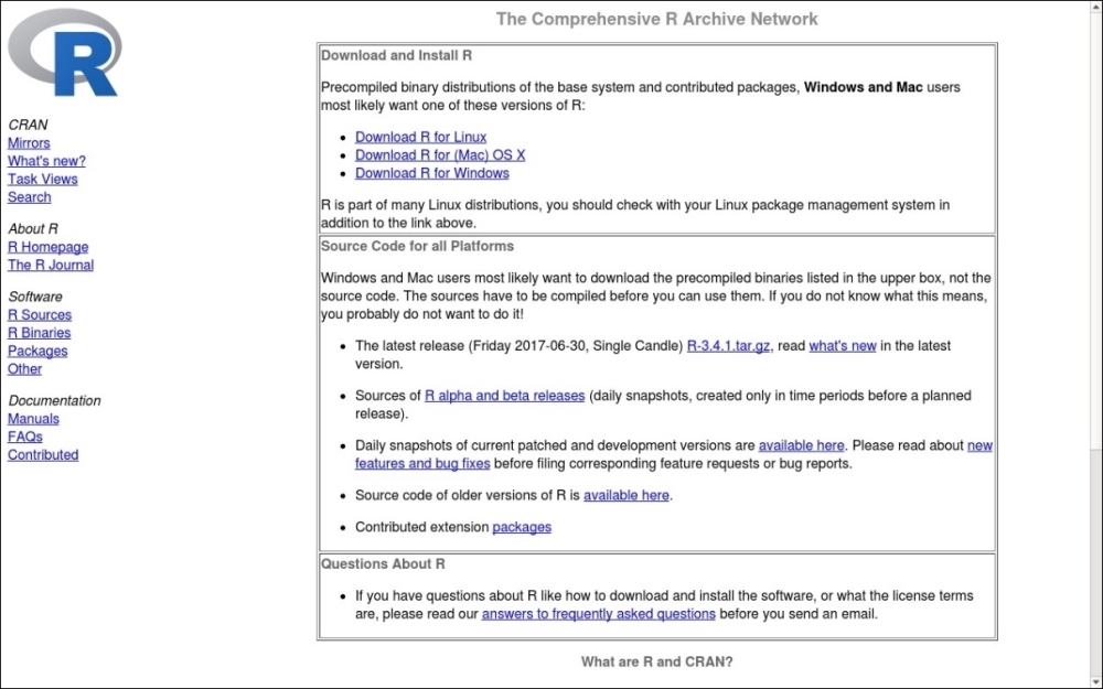
The CRAN Website (snapshot)
A Linux user may simply key in sudo apt-get install r-base in the Terminal, and post the return of the right password and privilege levels, and the R software would be installed. After the completion of the download and installation, the software is started by simply keying in R in the Terminal.
A Windows user needs to perform the following steps:
Firstly, click on Download R for Windows, as shown in the preceding screenshot.
Then in the base subdirectory click on install R for the first time.
In the new window, click on Download R 3.4.0 for Windows and download the
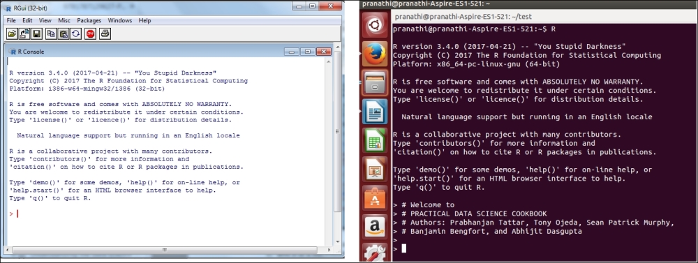
.exefile to a directory of your choice.The completely downloaded
R-3.0.0-win.exefile can be installed as any other.exefile.The R software may be invoked either from the Start menu, or from the icon on the desktop. The installed versions of R in Windows and Linux appears as follows:
The CRAN repository hosts 10,969 packages as of July 2, 2017. The packages are written and maintained by statisticians, engineers, biologists, and others. The reasons are varied and the resourcefulness is very rich and it reduces the need of writing exhaustive and new functions and programs from scratch. These additional packages can be obtained from https://cran.r-project.org/web/packages/. The user can click on https://cran.rproject.org/web/packages/available_packages_by_date.html, which will direct you to a new web package. Let us illustrate the installation of an R package named gdata:
We now wish to install the
gdatapackage. There are multiple ways of completing this task:Clicking on the
gdatalabel leads to the web page: https://cran.r-project.org/web/packages/gdata/index.html.In this HTML file, we can find a lot of information about the package through Version, Depends, Imports, Published, Author, Maintainer, License, System Requirements, Installation, and CRAN checks.
Furthermore, the download options may be chosen from the package source, macOS X binary, and Windows binary, depending on whether the user’s OS is Unix, macOS, or Windows respectively.
Finally, a package may require other packages as a prerequisite, and it may itself be a prerequisite to other packages.
This information is provided in Reverse dependencies, Reverse depends, Reverse imports, and Reverse suggests.
Suppose that the user has Windows OS. There are two ways to install the
gdatapackage:Start R, as explained earlier. At the console, execute the code
install.packages("gdata”).A CRAN mirror window will pop-up, asking the user to select one of the available mirrors.
Select one of the mirrors from the list. You may need to scroll down to locate your favorite mirror, and then hit the Ok button.
A default setting is
dependencies=TRUE, which will then download and install all the other required packages.Unless there are some violations, such as the dependency requirement of the R version being at least 2.3 in this case, the packages would be installed successfully.
A second way of installing the
gdatapackage is as follows:At the
gdataweb page, click on the following link: gdata_2.18.0.zip.This action will then attempt to download the package through the File download window.
Choose the option Save and specify the path where you wish to download the package.
In my case, I have chosen the
C:\Users\author\Downloadsdirectory.Now go to the R windows. In the menu ribbon, we have seven options in File, Edit, View, Misc, Packages, Windows, and Help.
Yes, your guess is correct and you would have wisely selected Packages from the menu.
Now, select the last option of Packages in Install Package(s) from local zip files and direct it to the path where you have downloaded the ZIP file.
Select the
gdata_2.18.0file and R will do the required remaining part of installing the package.
The one drawback of doing this process manually is that if there are dependencies, the user needs to ensure that all such packages have been installed before embarking on this second task of installing the R packages. However, despite this problem, it is quite useful to know this technique, as we may not be connected to the internet all the time, and we can install the packages when it is convenient.
This book uses lot of datasets from the web, statistical text books, and so on. The file format of the datasets have been varied and thus to help the reader, we have put all the datasets used in the book in an R package, RSADBE, which is the abbreviation of this book’s title. This package will be available from the CRAN website as well as this book’s web page. Thus, whenever you are asked to run data(xyz), the dataset xyz will be available either in the RSADBE package or datasets package of R.
The book also uses many of the packages available on CRAN. The following table gives the list of packages and the reader is advised to ensure that these packages are installed before you begin reading the chapter. That is, the reader needs to ensure that, as an example, install.packages(c("qcc”,”ggplot2”)) is run in the R session before proceeding with Chapter 3, Data Visualization.
|
Chapter number |
Packages required |
|---|---|
|
2 |
|
|
3 |
|
|
4 |
|
|
5 |
|
|
6 |
|
|
7 |
|
|
8 |
|
|
9 |
|
|
10 |
|
The major change in the second edition is augmenting the book with parallel Python programs. The reader might ask the all-important one word question Why? A simple reason, among others, is this: R has an impressive 11,212 packages, and the quantum of impressiveness for Python’s 11,4368 is left to the reader.
Of course, it is true that not all of these Python packages are related to data analytics. The number of packages is as of the date August 11, 2017. Importantly, the purpose of this book is to help the R user learn Python easily and vice versa. The main source of Python would be its website: https://www.python.org/:
Version- A famous argument debated among Python users is related to the choice of version 2.7 or 3.4+. Though the 3.0 version has been available since a decade earlier from 2008, the 2.7 version is still too popular and shows no signs of fading away. We will not get into the pros and cons of using the versions and will simply use the 3.4+ version. The author has run the programs in 3.4 version Ubuntu and 3.6 version in Windows and the code ran without any problems. The users of the 2.7 version might be disappointed, though we are sure that they can easily adapt it to their machines. Thus, we are providing the code for the 3.4+ version of Python.
Ubuntu OS already has Python installed and the version that comes along with it is 2.7.13-2. The two lines of code can be run in the gnome-terminal to update Python to the 3.6 version:
sudo apt-get update
sudo apt-get install python3.6
The Windows version can be easily downloaded from https://www.python.org/downloads/ and for making good use of the book code, the user is recommended to use the current version 3.6. The exe files don’t need an explanation. The snippets of Python software after they are started in Ubuntu and Windows are given next:
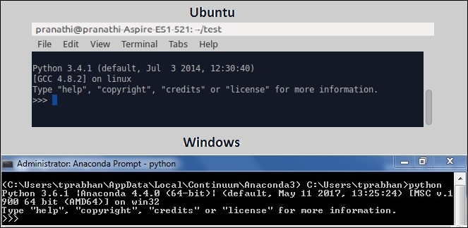
Simple arithmetic operations are easily carried out in Python. The user can key-in 2+7 at the prompt. Important programming will be taken up soon and the user can learn them from scratch from the next chapter.
Additional packages as required need to be installed separetely. pip is the package manager for Python. If any software is required, we can run the following line as the Python prompt:
pip install package
The table of packages required according to the chapters is given in the following table:
|
Chapter number |
Python Packages |
|---|---|
|
2 |
|
|
3 |
|
|
4 |
|
|
5 |
|
|
6 |
|
|
7 |
|
|
8 |
|
|
9 |
|
|
10 |
|
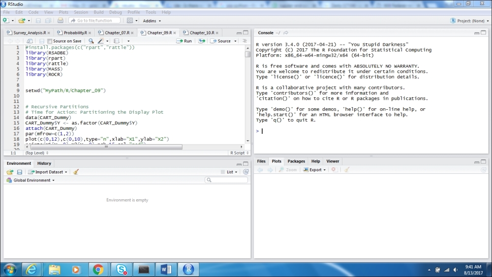
The Integrated Development Environment or IDE- most users do not use the software frontend these days. IDEs are convenient for many reasons and the uninitiated reader can search for the keyword. In very simple terms, the IDE may be thought of as the showroom and the core software as the factory. The RStudio appears to be the most popular IDE for R and Jupyter Notebook for Python.
The website for RStudio is https://www.rstudio.com/ and for Jupyter Notebook, it is http://jupyter.org/. The authors of the RStudio version are shown in the following screenshot:
We will not delve into details on the IDEs and the role they play. It is good enough to use them. More details about the importance of IDEs can be easily obtained on the web, and especially Wikipedia. An important Python distribution is Anaconda and there are lots of funny stories about the Anaconda-Python predators and how their names fascinate the software programmers. The Anaconda distribution is available at https://www.continuum.io/downloads and we recommend the reader to use the same. All the Python programs are run on the Jupyter Notebook IDE. The authors of the Anaconda Prompt are shown in the following screenshot:
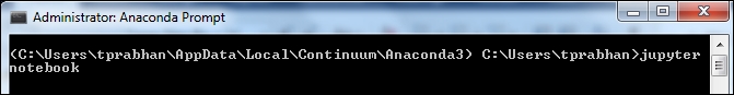
The code in the jupyter notebook has not yet run. And if you enter that on your Anaconda Prompt and hit the return key, the IDE will be started. The frontend of the Jupyter notebook, which will be opened in your default internet browser, looks like the following:
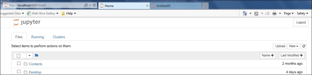
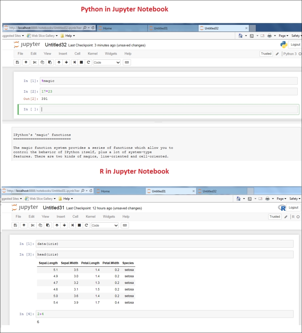
Now, an important question is the need of different IDEs for different software. Of course, it is not necessary. The R software can be integrated with the Anaconda distribution, particularly with options later in the Jupyter IDE. Towards this, we need to run the code conda install -c r r-essentials in the Anaconda Prompt. Now, if you click on the New drop-down button, you will see two options under the Notebook: one is Python 3 and the other is R. Thus, you can now run Python as well as R in the Jupyter Notebook IDE:
Python Idle is also another popular IDE and the Windows version looks like this:

After the user downloads the code bundle, RPySADBE.zip, from the publisher’s website, the first task is to unzip it to a local machine. We encourage the reader to download the code bundle since the R and Python code in the ebook might be in image format and it is a futile exercise to key in long programs all over again.
The folder structure in the unzipped format will consist of two folders: R and Python. Each of these chapters further consists of 10 sub-folders, one folder for each chapter. R software has a special package for itself as RSADBE available on CRAN. Thus, it does not have a Data sub-folder with the exception of Chapter 2, Import/Export Data. The chapter level folders for R will contain two sub-folders: Output and SRC. The SRC folder contains a file named Chapter_Number.R, which consists of all code used in the package. The Output folder contains a Microsoft Word document named Chapter_Number.doc. The reader is given an exercise to set up the Markdown settings; search for it on the web. The Chapter_Number.doc is the result of running the R file Chapter_Number.R. The graphics in the Markdown files will be different from the ones observed in the book.
Python’s chapter sub-folders are of three types: Data, Output, SRC. The required Comma Separated Values (CSV) data files are available in the Data folder while the SRC folder consists of the Python code file, Chapter_Number.py. The output file as a consequence of running the Python file in the IDE is saved as a Chapter_Number_Title.ipynb file. In many cases, the graphics generated by either R or Python for the same purpose yields the same display.
Since the R software has been run first and the explanation with the interpretation given following it, we have given the corresponding Python program, which is different; the graphical output is not necessarily produced in the book. In such cases, the ipynb files would come in handy as they contain all the graphics. Markdown is available for Python too, but we don’t pursue it though.
Here’s a final word about executing the R and Python files. The author does not have access about the path of the unzipped folder. Thus, the reader needs to specify the path appropriately in the R and Python files. Most likely, the reader would have to replace MyPath by /home/user/RPySADBE or C:/User/Documents/RPySADBE.
We will now begin formal discussion of the essential probability distributions.
The previous section highlights the different forms of variables. The variables such as Gender, Car_Model, and Minor_Problems possibly take one of the finite values. These variables are particular cases of the more general class of discrete variables.
It is to be noted that the sample space of a discrete variable need not be finite. As an example, the number of errors on a page may take values on the set of positive integers, {0, 1, 2, …}. Suppose that a discrete random variable X can take values among  with respective probabilities
  , that is,
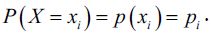 . Then, we require that the probabilities be non-zero and further that their sum be 1:
where the Greek symbol  represents summation over the index i.
The function  is called the probability mass function (pmf) of the discrete RV X. We will now consider formal definitions of important families of discrete variables. The engineers may refer to Bury (1999) for a detailed collection of useful statistical distributions in their field. The two most important parameters of a probability distribution are specified by mean and variance of the RV X.
In some cases, and important too, these parameters may not exist for the RV. However, we will not focus on such distributions, though we caution the reader that this does not mean that such RVs are irrelevant. Let us define these parameters for the discrete RV. The mean and variance of a discrete RV are respectively calculated as:
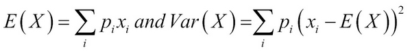
The mean is a measure of central tendency, whereas the variance gives a measure of the spread of the RV.
The variables defined so far are more commonly known as categorical variables. Agresti (2002) defines a categorical variable as a measurement scale consisting of a set of categories.
Let us identify the categories for the variables listed in the previous section. The categories for the Gender variable are male and female; whereas the car category variables derived from Car_Model are hatchback, sedan, station wagon, and utility vehicles. The Minor_Problems and Major_Problems variables have common but independent categories, yes and no; and, finally, the Satisfaction_Rating variable has the categories, as seen earlier, Very Poor, Poor, Average, Good, and Very Good. The Car_Model variable is just a set of labels of the name of car and it is an example of a nominal variable.
Finally, the output of the Satistifaction_Rating variable has an implicit order in it: Very Poor < Poor < Average < Good < Very Good. It may be apparent that this difference poses subtle challenges in their analysis. These types of variables are called ordinal variables. We will look at another type of categorical variable that has not popped up thus far.
Practically, it is often the case that the output of a continuous variable is put in a certain bin for ease of conceptualization. A very popular example is the categorization of the income level or age. In the case of income variables, it has become apparent in one of the earlier studies that people are very conservative about revealing their income in precise numbers.
For example, the author may be shy to reveal that his monthly income is Rs. 34,892. On the other hand, it has been revealed that these very same people do not have a problem in disclosing their income as belonging to one of the following categories: < Rs. 10,000, Rs. 10,000-30,000, Rs. 30,000-50,000, and > Rs. 50,000. Thus, this information may also be coded into labels and then each of the labels may refer to any one value in an interval bin. Thus, such variables are referred as interval variables.
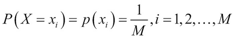
A random variable X is said to be a discrete uniform random variable if it can take any one of the finite M labels with equal probability.
As the discrete uniform random variable X can assume one of the 1, 2, …, M with equal probability, this probability is actually  . As the probability remains the same across the labels, the nomenclature uniform is justified. It might appear at the outset that this is not a very useful random variable. However, the reader is cautioned that this intuition is not correct. As a simple case, this variable arises in many cases where simple random sampling is needed in action. The pmf of a discrete RV is calculated as:
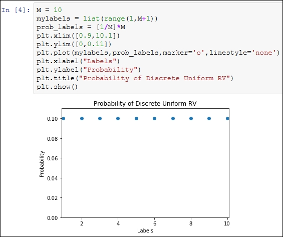
A simple plot of the probability distribution of a discrete uniform RV is demonstrated next:
> M = 10
> mylabels=1:M
> prob_labels=rep(1/M,length(mylabels))
> dotchart(prob_labels,labels=mylabels,xlim=c(.08,.12),
+ xlab=”Probability”)
> title("A Dot Chart for Probability of Discrete Uniform RV”)
Note
Downloading the example code
You can download the example code files for all Packt books you have purchased from your account at http://www.packtpub.com. If you purchased this book elsewhere, you can visit http://www.packtpub.com/support and register to have the files emailed directly to you.
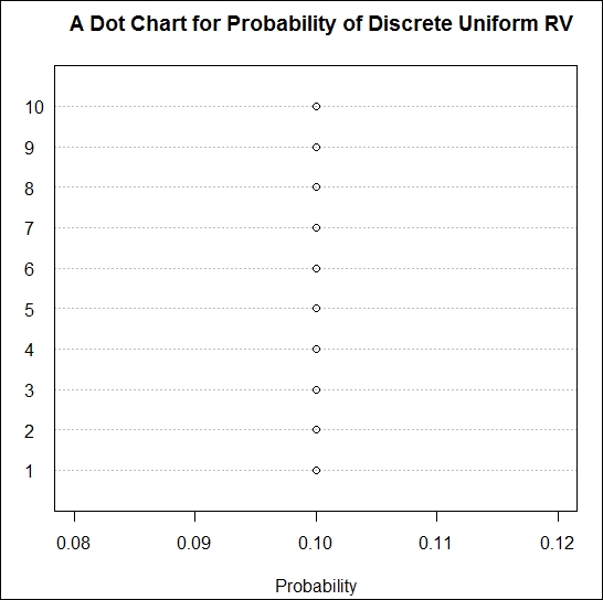
Probability distribution of a discrete uniform random variable
Note
The R programs here are indicative and it is not absolutely necessary that you follow them here. The R programs will actually begin from the next chapter and your flow won’t be affected if you do not understand certain aspects of them.
An equivalent Python program and its output is given in the following screenshot:
Recall the second question in the Experiments with uncertainty in computer science section, which asks: How many machines are likely to break down after a period of 1 year, 2 years, and 3 years?. When the outcomes involve uncertainty, the more appropriate question that we ask is related to the probability of the number of break downs being x.
Consider a fixed time frame, say 2 years. To make the question more generic, we assume that we have n number of machines. Suppose that the probability of a breakdown for a given machine at any given time is p. The goal is to obtain the probability of x machines with the breakdown, and implicitly (n-x) functional machines. Now consider a fixed pattern where the first x units have failed and the remaining are functioning properly. All the n machines function independently of other machines. Thus, the probability of observing x machines in the breakdown state is  .
.
Similarly, each of the remaining (n-x) machines have the probability of (1-p) of being in the functional state, and thus the probability of these occurring together is  . Again, by the independence axiom value, the probability of x machines with a breakdown is then given by
 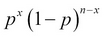 . Finally, in the overall setup, the number of possible samples with a breakdown being x and (n-x) samples being functional is actually the number of possible combinations of choosing x-out-of-n items, which is the combinatorial
  .
.
As each of these samples is equally likely to occur, the probability of exactly x broken machines is given by 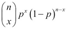 . The RV X obtained in such a context is known as the binomial RV and its pmf is called as the binomial distribution. In mathematical terms, the pmf of the binomial RV is calculated as:
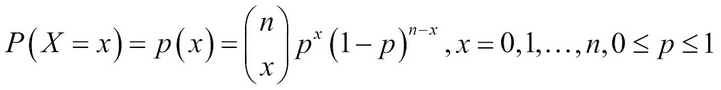
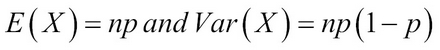
The pmf of a binomial distribution is sometimes denoted by  . Let us now look at some important properties of a binomial RV. The mean and variance of a binomial RV X are respectively calculated as:
Note
As p is always a number between 0 and 1, the variance of a binomial RV is always lesser than its mean.
Example 1.3.1: Suppose n = 10 and p = 0.5. We need to obtain the probabilities p(x), x=0, 1, 2, …, 10. The probabilities can be obtained using the built-in R function, dbinom. The function dbinom returns the probabilities of a binomial RV.
The first argument of this function may be a scalar or a vector according to the points at which we wish to know the probability. The second argument of the function needs to know the value of n, the size of the binomial distribution. The third argument of this function requires the user to specify the probability of success in p. It is natural to forget the syntax of functions and the R help system becomes very handy here. For any function, you can get details of it using ? followed by the function name. Please do not insert a space between ? and the function name. Here, you can try ?dbinom:
> n <- 10; p <- 0.5
> p_x <- round(dbinom(x=0:10, n, p),4)
> plot(x=0:10,p_x,xlab=”x”, ylab=”P(X=x)”)
The R function round fixes the accuracy of the argument up to the specified number of digits.
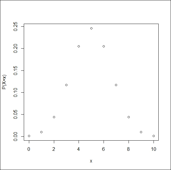
Binomial probabilities
We have used the dbinom function in the previous example. There are three utility facets for the binomial distribution. The three facets are p, q, and r. These three facets respectively help us in computations related to cumulative probabilities, quantiles of the distribution, and simulation of random numbers from the distribution. To use these functions, we simply augment the letters with the distribution name, binom, here, as pbinom, qbinom, and rbinom. There will be, of course, a critical change in the arguments. In fact, there are many distributions for which the quartet of d, p, q, and r are available; check ?Distributions.
The Python code block is the following:
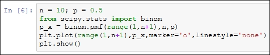
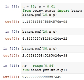
Example 1.3.2: Assume that the probability of a key failing on an 83-set keyboard (the authors, laptop keyboard has 83 keys) is 0.01. Now, we need to find the probability when at a given time there are 10, 20, and 30 non-functioning keys on this keyboard. Using the dbinom function, these probabilities are easy to calculate. Try to do this same problem using a scientific calculator or by writing a simple function in any language that you are comfortable with:
> n <- 83; p <- 0.01
> dbinom(10,n,p)
[1] 1.168e-08
> dbinom(20,n,p)
[1] 4.343e-22
> dbinom(30,n,p)
[1] 2.043e-38
> sum(dbinom(0:83,n,p))
[1] 1
As the probabilities of 10-30 keys failing appear too small, it is natural to believe that maybe something is going wrong. As a check, the sum clearly equals 1. Let us have a look at the problem from a different angle. For many x values, the probability p(x) will be approximately zero. We may not be interested in the probability of an exact number of failures though we are interested in the probability of at least x failures occurring, that is, we are interested in the cumulative probabilities  . The cumulative probabilities for binomial distribution are obtained in R using the
 pbinom function. The main arguments of pbinom include size (for n), prob (for p), and q (the at least x argument). For the same problem, we now look at the cumulative probabilities for various p values:
> n <- 83; p <- seq(0.05,0.95,0.05)
> x <- seq(0,83,5)
> i <- 1
> plot(x,pbinom(x,n,p[i]),”l”,col=1,xlab=”x”,ylab=
+ expression(P(X<=x)))
> for(i in 2:length(p)) { points(x,pbinom(x,n,p[i]),”l”,col=i)}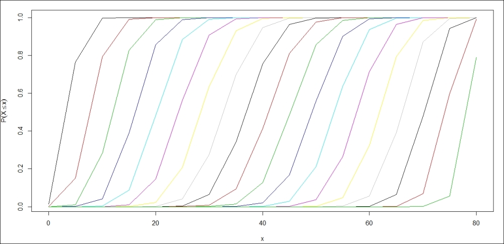
Cumulative binomial probabilities
Try to interpret the preceding figure, the parallel Python program would be the following:
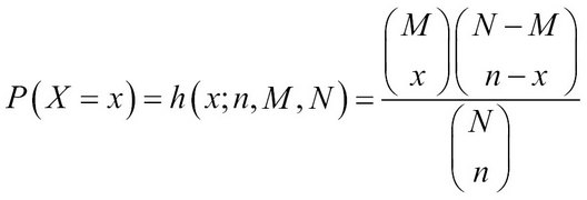
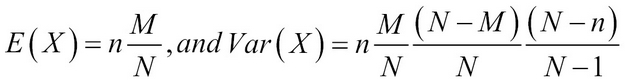
A box of N = 200 pieces of 12 GB pen drives arrives at a sales center. The carton contains M = 20 defective pen drives. A random sample of n units is drawn from the carton. Let X denote the number of defective pen drives obtained from the sample of n units. The task is to obtain the probability distribution of X. The number of possible ways of obtaining the sample of size n is  . In this problem, we have M defective units and N-M working pen drives, and x defective units can be sampled in
  different ways and n-x good units can be obtained in
  distinct ways. Thus, the probability distribution of the RV X is calculated as:
where x is an integer between 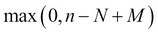 and
and  . The RV is called the hypergeometric RV and its probability distribution is called the hypergeometric distribution.
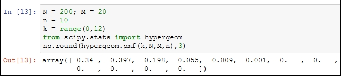
Suppose that we draw a sample of n = 10 units. The dhyper function in R can be used to find the probabilities of the RV X, assuming different values:
> N = 200; M = 20
> n = 10
> x = 0:11
> round(dhyper(x,M,N,n),3)
 [1] 0.377 0.395 0.176 0.044 0.007 0.001 0.000 0.000 0.000 0.000 0.000 0.000
The equivalent Python implementation is as follows:
The mean and variance of a hypergeometric distribution are stated as follows:
Consider a variant of the problem described in the previous subsection. The 10 new desktops need to be fitted with an add-on, five megapixel external cameras, to help the students attend a certain online course. Assume that the probability of a non-defective camera unit is p. As an administrator, you keep on placing orders until you receive 10 non-defective cameras. Now, let X denote the number of orders placed for obtaining the 10 good units. We denote the required number of successes by k, which in this discussion has been k = 10. The goal in this unit is to obtain the probability distribution of X.
Suppose that the xth order placed results in the procurement of a kth non-defective unit. This implies that we have received (k-1) non-defective units among the first (x-1) orders placed, which is possible in  distinct ways. At the xth order, the instant of having received the kth non-defective unit, we have k successes and x-k failures. Thus, the probability distribution of the RV is calculated as:
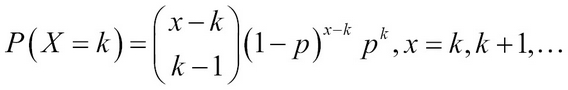
Such an RV is called a negative binomial RV and its probability distribution as the negative binomial distribution. Technically, this RV has no upper bound as the next required success may never turn up. We state the mean and variance of this distribution as follows:
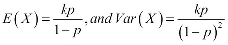
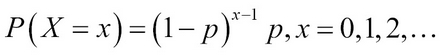
A particular and important special case of the negative binomial RV occurs for k = 1, which is known as the geometric RV. In this case, the pmf is calculated as:
Example 1.3.3. (Baron (2007). Page 77) sequential testing: In a certain setup, the probability of an item being defective is (1-p) = 0.05. To complete the lab setup, 12 non-defective units are required. We need to compute the probability that at least 15 units need to be tested. Here we make use of the cumulative distribution of the negative binomial distribution pnbinom function available in R. Similar to the pbinom function, the main arguments that we require here would be size, prob, and q. This problem is solved in a single line of code:
> 1-pnbinom(3,size=12,0.95)
[1] 0.005467259
Note that we have specified 3 as the quantile point (at least x argument) as the size parameter of this experiment is 12 and we are seeking at least 15 units that translate into three more units than the size of the parameter. The pnbinom function computes the cumulative distribution function and the requirement is actually the complement and hence the expression in the code is 1–pnbinom. We may equivalently solve the problem using the dnbinom function, which straightforwardly computes the required probability:
> 1-(dnbinom(3,size=12,0.95)+dnbinom(2,size=12,0.95)+dnbinom(1,
+ size=12,0.95)+dnbinom(0,size=12,0.95))
[1] 0.005467259
The number of accidents on a 1 km stretch of road, the total calls received during a 1-hour slot on your mobile, the number of "likes” received on a status on a social networking site in a day, and similar other cases, are some of the examples that are addressed by the Poisson RV. The probability distribution of a Poisson RV is calculated as:
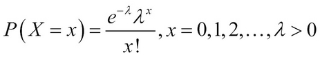
Here,  is the parameter of the Poisson RV with X denoting the number of events. The Poisson distribution is sometimes also referred to as the law of rare events. The mean and variance of the Poisson RV are surprisingly the same and equal , that is,
 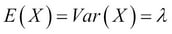 .
.
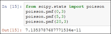
Example 1.3.4: Suppose that Santa commits errors in a software program with a mean of three errors per A4-size page. Santa’s manager wants to know the probability of Santa committing 0, 5, and 20 errors per page. The R function, dpois, helps to determine the answer:
> dpois(0,lambda=3); dpois(5,lambda=3); dpois(20, lambda=3)
[1] 0.04978707
[1] 0.1008188
[1] 7.135379e-11
Note that Santa’s probability of committing 20 errors is almost 0.The Python program is the following:
We will next focus on continuous distributions.
The numeric variables in the survey, Age, Mileage, and Odometer, can take any values over a continuous interval and these are examples of continuous RVs. In the previous section, we dealt with RVs that had discrete output. In this section, we will deal with RVs that have continuous output. A distinction from the previous section needs to be pointed out explicitly.
In the case of a discrete RV, there is a positive number for the probability of an RV taking on a certain value that is determined by the pmf. In the continuous case, an RV necessarily assumes any specific value with zero probability. These technical issues cannot be discussed in this book. In the discrete case, the probabilities of certain values are specified by the pmf, and in the continuous case the probabilities, over intervals, are decided by the probability density function, abbreviated as pdf.
Suppose that we have a continuous RV X with the pdf f(x) defined over the possible x values; that is, we assume that the pdf f(x) is well defined over the range of the RV X, denoted by  . It is necessary that the integration of f(x) over the range is necessarily 1; that is,
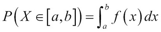
 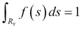 .The probability that the RV X takes a value in an interval [a, b] is defined by:
In general, we are interested in the cumulative probabilities of a continuous RV, which is the probability of the event P(X<x). In terms of the previous equations, this is obtained as:
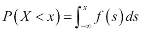
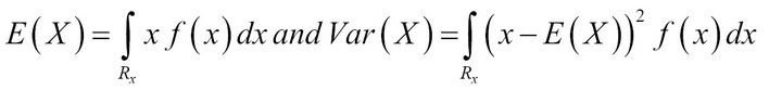
A special name for this probability is the cumulative density function. The mean and variance of a continuous RV are then defined by:
As in the previous section, we will begin with the simpler RV in uniform distribution.
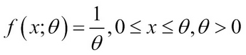
A RV is said to have uniform distribution over the interval  if its probability density function is given by:
In fact, it is not necessary to restrict our focus on the positive real line. For any two real numbers a and b, from the real line, with b > a, the uniform RV can be defined by:
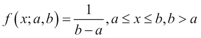
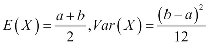
The uniform distribution has a very important role to play in simulation, as will be seen in Chapter 6, Simulation. As with the discrete counterpart, in the continuous case any two intervals of the same length will have an equal probability occurring. The mean and variance of a uniform RV over the interval [a, b] are respectively given by:
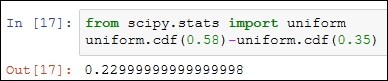
Example 1.4.1. Horgan’s (2008), Example 15.3: The International Journal of Circuit Theory and Applications reported in 1990 that researchers at the University of California, Berkeley, had designed a switched capacitor circuit for generating random signals whose trajectory is uniformly distributed over the unit interval [0, 1]. Suppose that we are interested in calculating the probability that the trajectory falls in the interval [0.35, 0.58]. Though the answer is straightforward, we will obtain it using the punif function:
> punif(0.58)-punif(0.35)
[1] 0.23
Of course, we don’t need software for such simple integrals, nevertheless:
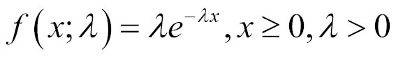
The exponential distribution is probably one of the most important probability distributions in statistics, and more so for computer scientists. The numbers of arrivals in a queuing system, the time between two incoming calls on a mobile, the lifetime of a laptop, and so on, are some of the important applications where this distribution has a lasting utility value. The pdf of an exponential RV is specified by:
The parameter is sometimes referred to as the failure rate. The exponential RV enjoys a special property called the memory-less property, which conveys that: 
The mathematical statement translates into the property that if X is an exponential RV, then its failure in the future depends on the present, and the past (age) of the RV does not matter. In simple words, this means that the probability of failure is constant in time and does not depend on the age of the system. Let us obtain the plots of a few exponential distributions:
> par(mfrow=c(1,2))
> curve(dexp(x,1),0,10,ylab=”f(x)”,xlab=”x”,cex.axis=1.25)
> curve(dexp(x,0.2),add=TRUE,col=2)
> curve(dexp(x,0.5),add=TRUE,col=3)
> curve(dexp(x,0.7),add=TRUE,col=4)
> curve(dexp(x,0.85),add=TRUE,col=5)
> legend(6,1,paste("Rate = ",c(1,0.2,0.5,0.7,0.85)),col=1:5,pch=
+ "___”)
> curve(dexp(x,50),0,0.5,ylab=”f(x)”,xlab=”x”)
> curve(dexp(x,10),add=TRUE,col=2)
> curve(dexp(x,20),add=TRUE,col=3)
> curve(dexp(x,30),add=TRUE,col=4)
> curve(dexp(x,40),add=TRUE,col=5)
> legend(0.3,50,paste("Rate = ",c(1,0.2,0.5,0.7,0.85)),col=1:5,pch=
+ "___”)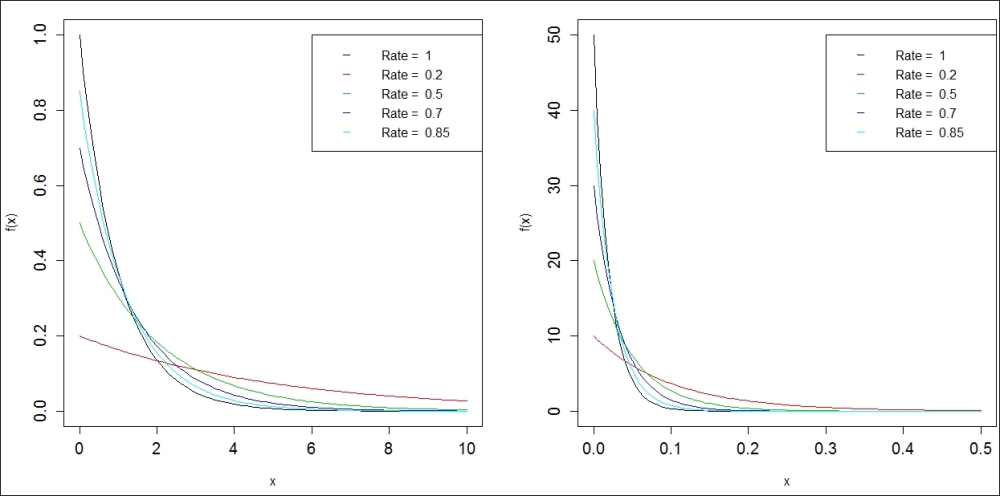
The exponential densities
The mean and variance of this exponential distribution are listed as follows:
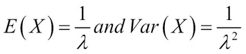
The complete Python code block is given next:
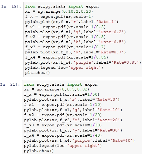
The normal distribution is in some sense an all-pervasive distribution that arises sooner or later in almost any statistical discussion. In fact, it is very likely that the reader may already be familiar with certain aspects of the normal distribution; for example, the shape of a normal distribution curve is bell-shaped. The mathematical appropriateness is probably reflected through the reason that though it has a simpler expression, its density function includes the three most famous irrational numbers 
Suppose that X is normally distributed with the mean  and the variance
  . Then, the probability density function of the normal RV is given by:

If the mean is zero and the variance is 1, the normal RV is referred to as the standard normal RV, and the standard is to denote it by Z.
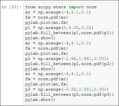
Example 1.4.2. Shady Normal Curves: We will again consider a standard normal random variable, which is more popularly denoted in Statistics by Z. Some of the most needed probabilities are P(Z > 0) and P(-1.96 < Z < 1.96). These probabilities are now shaded:
> par(mfrow=c(3,1))
> # Probability Z Greater than 0
> curve(dnorm(x,0,1),-4,4,xlab=”z”,ylab=”f(z)”)
> z=seq(0,4,0.02)
> lines(z,dnorm(z),type=”h”,col=”grey”)
> # 95% Coverage
> curve(dnorm(x,0,1),-4,4,xlab=”z”,ylab=”f(z)”)
> z=seq(-1.96,1.96,0.001)
> lines(z,dnorm(z),type=”h”,col=”grey”)
> # 95% Coverage
> curve(dnorm(x,0,1),-4,4,xlab=”z”,ylab=”f(z)”)
> z=seq(-2.58,2.58,0.001)
> lines(z,dnorm(z),type=”h”,col=”grey”)
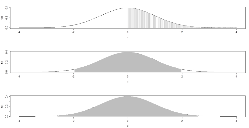
Shady normal curves
The Python program for the shady normal probabilities is given next:
The reader should now be clear with the distinct nature of variables that arise in different scenarios. In R, the reader should be able to verify that the data is in the correct format. Furthermore, the important families of random variables are introduced in this chapter, which should help the reader in dealing with them when they crop up in their experiments. Computation of simple probabilities were also introduced and explained.
In the next chapter, the reader will learn how to perform the basic R computations, creating data objects, and so on. As data can seldom be constructed completely in R, we need to import data from external foreign files. The methods explained help the reader to import data in file formats such as .csv and .xls. Similar to importing, it is also important to be able to export data/output to other software. Finally, the R session management will conclude the next chapter.


